University of Warwick institutional repository: http://go.warwick.ac.uk/wrap
A Thesis Submitted for the Degree of PhD at the University of Warwick
http://go.warwick.ac.uk/wrap/3759
This thesis is made available online and is protected by original copyright.
Please scroll down to view the document itself.
AUTHOR:Tao Li DEGREE: Ph.D.
TITLE: Relational Clustering Models for Knowledge Discovery and Recommender Systems
DATE OF DEPOSIT: . . . .
I agree that this thesis shall be available in accordance with the regulations governing the University of Warwick theses.
I agree that the summary of this thesis may be submitted for publication.
Iagreethat the thesis may be photocopied (single copies for study purposes only). Theses with no restriction on photocopying will also be made available to the British Library for microfilming. The British Library may supply copies to individuals or libraries. subject to a statement from them that the copy is supplied for non-publishing purposes. All copies supplied by the British Library will carry the following statement:
“Attention is drawn to the fact that the copyright of this thesis rests with its author. This copy of the thesis has been supplied on the condition that anyone who consults it is understood to recognise that its copyright rests with its author and that no quotation from the thesis and no information derived from it may be published without the author’s written consent.”
AUTHOR’S SIGNATURE: . . . .
USER’S DECLARATION
1. I undertake not to quote or make use of any information from this thesis without making acknowledgement to the author.
2. I further undertake to allow no-one else to use this thesis while it is in my care.
DATE SIGNATURE ADDRESS
. . . .
. . . .
. . . .
. . . .
M A E
G
NS I
T A T MOLEM
U N
IV
ER
SITAS WARWICEN SIS
Relational Clustering Models for Knowledge Discovery
and Recommender Systems
by
Tao Li
Thesis
Submitted to the University of Warwick
for the degree of
Doctor of Philosophy
Contents
List of Tables v
List of Figures vi
Acknowledgments ix
Declarations xi
Abstract xii
Chapter 1 Preface 1
I Relational Clustering 5
Chapter 2 Review of Relational Clustering 8
2.1 Fundamentals of Relational Clustering . . . 13
2.1.1 Relational Data . . . 13
2.1.2 Proximity Measures . . . 17
2.1.3 Evaluation Criteria . . . 25
2.1.4 Determining the Number of Clusters . . . 27
2.2 Relational Clustering Algorithms . . . 29
2.2.1 Proximity-based Clustering . . . 29
2.2.3 Model-based Clustering . . . 32
2.2.4 Graph-based Clustering . . . 34
2.2.5 Spectral Clustering . . . 35
2.2.6 Fuzzy Clustering . . . 36
2.2.7 Constraint-based Clustering . . . 37
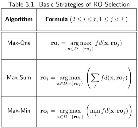
Chapter 3 Representative Objects 39 3.1 Representative Objects . . . 40
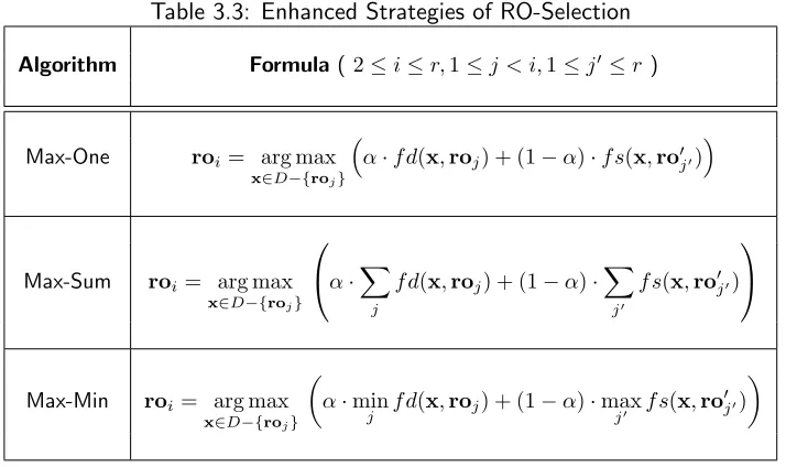
3.2 Extension of RO-Selection Strategies . . . 45
3.2.1 Discriminate different data clusters . . . 46
3.2.2 Determine ROs incrementally . . . 50
3.3 Summary . . . 55
Chapter 4 DIVA Clustering Framework 56 4.1 Divisive Step . . . 57
4.1.1 Recursive Approach . . . 57
4.1.2 Incremental Approach . . . 60
4.2 Agglomerative Step . . . 63
4.3 Complexity Analysis . . . 65
4.4 Experiments on Propositional Datasets . . . 67
4.4.1 Arbitrary-shaped Dataset . . . 68
4.4.2 UCI Chess Dataset . . . 70
4.5 Experiments on Relational Datasets . . . 71
4.5.1 Synthetic Amazon Dataset . . . 72
4.5.2 DBLP Dataset . . . 75
4.5.3 Movie Dataset . . . 78
II Automated Taxonomy Generation 83
Chapter 5 Review of Taxonomy Generation Algorithms 86
5.1 Fundamentals of the ATG algorithms . . . 87
5.2 Evaluation Criteria . . . 91
Chapter 6 Taxonomy Generation for Relational Datasets 93 6.1 Search Model for Learning . . . 93
6.2 Taxonomy Construction . . . 94
6.2.1 Global-Cut . . . 96
6.2.2 Local-Cut . . . 100
6.3 Complexity Analysis . . . 101
6.4 Experiments . . . 103
6.4.1 Synthetic Amazon Dataset . . . 105
6.4.2 Real Dataset . . . 107
6.5 Summary . . . 111
Chapter 7 Labeling the Automatically Generated Taxonomic Nodes 113 7.1 Labeling Strategies . . . 114
7.2 Experimental Results . . . 118
7.2.1 Bias within Kullback-Liebler Divergence . . . 118
7.2.2 Empirical Study . . . 119
7.3 Summary . . . 121
7.4 Appendix . . . 123
7.4.1 Proof of the KL-divergence Bounds . . . 123
III Recommender Systems 125
Chapter 8 Review of Recommender Systems 129
8.1 Fundamentals of Recommender Systems . . . 129
8.2 Exploitation of Domain Knowledge to Improve the Recommendation Quality . . . 131
8.3 Utilization of Data Mining Techniques to Improve the System Scalability 133 8.4 Proximity Measure based on Taxonomy . . . 134
Chapter 9 Exploitation of Taxonomy in Recommender Systems 136 9.1 Framework of Recommender System . . . 136
9.2 Integration of Taxonomies . . . 141
9.2.1 Preserve Item Similarities . . . 141
9.2.2 Group User Visits . . . 144
9.3 Experimental Results . . . 144
9.3.1 Movie Retailer . . . 146
9.3.2 MovieLens . . . 148
9.4 Summary . . . 150
List of Tables
2.1 Propositional Iris Dataset . . . 13
2.2 Properties of distance functions . . . 17
2.3 Similarity Measure for Categorical dataset . . . 18
2.4 Linkage Matrix between Actors and Movies . . . 22
3.1 Basic Strategies of RO-Selection . . . 43
3.2 Basic Strategies of RO-Selection . . . 45
3.3 Enhanced Strategies of RO-Selection . . . 46
3.4 Incremental Strategies of RO-Selection . . . 53
3.5 Average Distance between ROs . . . 55
4.1 Execution Time of HAC, DBScan and DIVA (sec) . . . 69
4.2 Experimental Results on UCI Chess Dataset . . . 70
6.1 Experimental results using the Synthetic Amazon dataset . . . 106
6.2 Evaluation results using the movie dataset . . . 107
6.3 Taxonomy Nodes in Figure 6.3 with Corresponding Movies . . . 110
7.1 Bias of Different Attributes . . . 119
7.2 Results of Simulation Experiment . . . 121
List of Figures
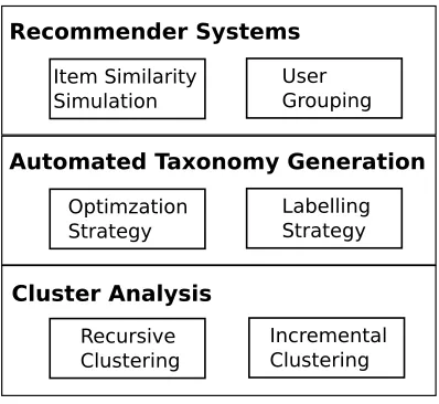
1.1 Our Research Framework . . . 3
2.1 Five Steps of Cluster Analysis . . . 9
2.2 Comparison of Flat and Hierarchical Clustering . . . 10
2.3 Schema of a movie dataset . . . 14
2.4 Example relational object for Tom Hanks . . . 16
2.5 Two Example Movie Stars . . . 21
2.6 Genre Taxonomy . . . 22
3.1 Comparison of RO-selection strategies . . . 44
3.2 RO-Selection Depending on Other Clusters . . . 46
3.3 Determine ROs to discriminate the clusters . . . 48
3.4 Dynamically update ROs . . . 52
3.5 Select ROs using incremental Max-Sum and Max-Min strategies . . . . 54
4.1 Cluster Results Using Different Strategy . . . 68
4.2 UCI Chess Dataset - Time Spent . . . 71
4.3 Ontology of the Synthetic Amazon dataset . . . 72
4.4 Synthetic Amazon Dataset - Clustering users w.r.t. different variance v 74 4.5 Synthetic Amazon Dataset - Clustering users w.r.t. different number of ROs . . . 76
4.7 Schema of the DBLP Database . . . 77
4.8 DBLP Dataset - Clustering authors w.r.t. different variancev . . . 79
4.9 Movie Dataset - Clustering movies w.r.t. different variancev . . . 81
6.1 Example of generating taxonomy . . . 99
6.2 Synthetic Amazon Dataset - Evaluate Taxonomy w.r.t noise . . . 107
6.3 Part of the Labeled Movie Taxonomy . . . 109
7.1 Example Taxonomy Sub-Tree . . . 115
7.2 Labeling Taxonomy for Movie Dataset . . . 122
9.1 Hierarchical taxonomy for preserving similarity values . . . 142
9.2 Recommendations for Movie Dataset based on Users . . . 147
9.3 Recommendations for Movie Dataset based on Sessions . . . 148
List of Algorithms
1 Iterative RO-Selection Procedure Using the Max-Sum Strategy . . . 49
2 Main Framework of DIVA . . . 57
3 RecDivStep . . . 58
4 IncDivaStep . . . 60
5 IncBuild . . . 61
6 AggStep . . . 65
7 Iterative Optimize the Taxonomic Structure . . . 98
8 Recursively Optimize the Taxonomic Structure . . . 102
9 CF-based Recommendation . . . 137
10 FindPair . . . 139
Acknowledgments
First of all, I would like to express my sincere gratitude to Dr. Sarabjot Singh Anand,
my supervisor at the University of Warwick. He has supported me in all his endeavors
and provided guidance throughout my PhD career. Besides, his insight and enthusiasm
in scientific research encourage me all the time.
I would also thank my advisor, Dr. Nathan Griffiths, for his invaluable comments
on my annual reports and PhD thesis. Thanks as well to Dr. Al´ıpio M. Jorge and
Dr. Sara Kalvala for their kind willingness to read and evaluate my dissertation.
As a member of the IAS group in the Department of Computer Science, I often
received constructive suggestions and technical support from other departmental staff, in
particular Dr. Alexandra Cristea, Dr. Mike Joy, Shanshan Yang, Jane Yau, Nick Landia,
Henry Franks, Maurice Hendrix, Fawaz Ghali, Dr. Sarah Lim Choi Keung, Dr. Charles
Care, Russell Boyatt, Dr. Zhan En (Eric) Chan, Shuangyan (Jenny) Liu, Dr. Christine
Leigh, Dr. Roger Packwood, Mr. Paul Williamson, Mr. Richard Cunningham, Mr. Rod
Moore, Ms. Catherine Pillet and Ms. Angie Cross. I would sincerely thank Prof. Stephen
Jarvis, Dr. Meurig Beynon, Prof. Kershaw Baz and Dr. Cherie Wang for their supervision
during my work as a teaching and research assistant.
My acknowledgement also goes to Prof. Hilary Marland, Ms. Ros Lucas, Dr. Joanne
Allen, Dr. Joanne Anderson, Dr. Chris Boyce, Dr. Jing Kang, Dr. Lorraine Lim, Dr. Lydia
Plath and Dr. Deborah Toner for the very pleasant atmosphere in the IAS semiars.
Last but by no means least, I would like to thank my best friends, Wee-Hoe
Liu, Dr. Ke Tang, Dr. Jie Bai, Dr. Zhi-Gang Zuo, Shuai Li, Wei-Dong Li, Jing-Long
Liu, Bo Wang, Jing-Bo Sun, Yu-Jia Xiang and others for their affection, support and
encouragement. Also I cannot forget my beloved parents for their unselfish love and
devotion, helping me in any conceivable respect. Finally, I want to thank Xiao (Grace)
Hu, for remind me that there are other important things in life besides machines and
algorithms.
Financial support has been provided by the Graduate School, the Department
of Computer Science and the Institute of Advanced Study in the University of
War-wick, through the schemes of Warwick Postgraduate Research Fellowship, Departmental
Declarations
This thesis is a presentation of my original research work. Wherever contributions of
others are involved, every effort is made to indicate this clearly, with due reference to
the literature, and acknowledgement of collaborative research and discussions. No part
of the work contained in this thesis has been submitted for any degree or qualification
at any other university.
Parts of this thesis were published previously in our papers: Chapter 2 extends
a state-of-the-art review of the relational clustering that was published in [92]. The
fundamental ideas of Chapters 3 and 4, including the recursive RO-selection algorithm as
well as the DIVA clustering framework, were first proposed in [89]. Later, the incremental
implementation of the DIVA framework was developed and reported in [88]. Chapters 6
and 7, which cover the techniques of automated taxonomy generation for relational data
and the algorithm of labeling taxonomic nodes by utilizing Kullback-Liebler Divergence,
were respectively published in [90] and [91]. Finally Chapter 9, i.e. the integration of
automatically derived taxonomy into the recommender systems, was published in [93].
Two journal papers are currently under preparation, which include the detailed results
Abstract
Cluster analysis is a fundamental research field in Knowledge Discovery and Data
Min-ing (KDD). It aims at partitionMin-ing a given dataset into some homogeneous clusters so as
to reflect the natural hidden data structure. Various heuristic or statistical approaches
have been developed for analyzing propositional datasets. Nevertheless, in relational
clustering the existence of multi-type relationships will greatly degrade the performance
of traditional clustering algorithms. This issue motivates us to find more effective
al-gorithms to conduct the cluster analysis upon relational datasets. In this thesis we
comprehensively study the idea of Representative Objects for approximating data
dis-tribution and then design a multi-phase clustering framework for analyzing relational
datasets with high effectiveness and efficiency.
The second task considered in this thesis is to provide some better data models for
people as well as machines to browse and navigate a dataset. The hierarchical taxonomy
is widely used for this purpose. Compared with manually created taxonomies,
automat-ically derived ones are more appealing because of their low creation/maintenance cost
and high scalability. Up to now, the taxonomy generation techniques are mainly used
to organize document corpus. We investigate the possibility of utilizing them upon
re-lational datasets and then propose some algorithmic improvements. Another non-trivial
problem is how to assign suitable labels for the taxonomic nodes so as to credibly
sum-marize the content of each node. Unfortunately, this field has not been investigated
sufficiently to the best of our knowledge, and so we attempt to fill the gap by proposing
The final goal of our cluster analysis and taxonomy generation techniques is
to improve the scalability of recommender systems that are developed to tackle the
problem of information overload. Recent research in recommender systems integrates
the exploitation of domain knowledge to improve the recommendation quality, which
however reduces the scalability of the whole system at the same time. We address this
issue by applying the automatically derived taxonomy to preserve the pair-wise
similari-ties between items, and then modeling the user visits by another hierarchical structure.
Experimental results show that the computational complexity of the recommendation
Chapter 1
Preface
Cluster analysis is an important research field in Knowledge Discovery and Data Mining
(KDD). The aim is to discover the intrinsic structure of the underlying dataset, which
is generally referred to as the unsupervised learning problem. This is different from
the supervised learning tasks (such as classification or regression) in which the data
model is first constructed from the training dataset and then to be applied upon the
test dataset. Many clustering algorithms have been proposed since the 1960s with
the utilization of various ideas in such fields as statistics, combinatorial mathematics,
artificial intelligence, spectral theory etc., but most of them are only suitable for analyzing
propositional datasets. In practice relational datasets that contain different data types
and relationships between them are more common. The existence of these multi-type
relationships greatly degrades the performance of the traditional clustering algorithms if
they are applied to the relational datasets naively. This issue motivates us to find more
effective algorithms to conduct cluster analysis upon the relational datasets.
After the cluster result has been obtained, a hierarchical taxonomy can be
gen-erated that provides a better mechanism for people to browse and navigate the dataset.
Automatically derived taxonomies are more appealing than manually derived ones
be-cause of their low creation/maintenance cost and high scalability. Generally speaking,
investigate the possibility of utilizing them upon relational datasets as well as propose
some algorithmic improvements. Another non-trivial problem is how to assign suitable
labels for the taxonomic nodes so as to help people more easily understand the content
of each node. Unfortunately, this field has not been investigated sufficiently to the best
of our knowledge, and so we attempt to fill the gap by proposing some novel approaches.
To validate their applicability in practice, we utilize our cluster analysis and
tax-onomy generation techniques within recommender systems. Recent research in this field
focuses on the incorporation of domain knowledge: meaningful neighbouring users are
identified based on the similarity of their visiting items, so the quality of user-based
recommendations will hopefully be improved as more relational domain information are
exploited during the item similarity computation. But as the tradeoff, the system
scala-bility is often decreased because exploiting such information needs more computational
effort than that of traditional recommender systems computing based on propositional
data. In this thesis, we propose to use an automatically derived taxonomy to preserve
the pair-wise similarities between items in an offline stage. These item similarities are
then retrieved directly from the taxonomy instead of obtained from the real-time
calcu-lation. By this way, the online computational expense of identifying neighbouring users
can be reduced and the system scalability be improved effectively. In addition, the user
visits are to be grouped within another hierarchical structure for further improving the
system scalability.
Figure 1.1 explains the layers of our research framework and the thesis is
orga-nized accordingly. We study relational clustering algorithms in Part I, which covers the
following chapters:
• Chapter 2 provides a comprehensive review of relational clustering, including some fundamental definitions and a categorization of different clustering algorithms with
a brief discussion of key algorithms;
Figure 1.1: Our Research Framework
strategies of identifying Representative Objects in the dataset;
• Chapter 4 proposes a multi-phase clustering framework that is especially efficient in analyzing relational datasets. Two implementations of the framework are
de-veloped that are suitable for static and incremental learning tasks respectively.
Then in Part II we turn to the automated taxonomy generation and discuss the following
topics:
• Chapter 5 reviews some important issues and related works in the field of auto-mated taxonomy generation;
• Chapter 6 explains our taxonomy generation algorithm that is developed from the relational clustering framework;
• Chapter 7 discusses our approach of assigning labels for taxonomic nodes based on the idea of Kullback-Liebler Divergence.
After that, in Part III we will investigate the application of our data mining techniques
in practice, i.e. to improve the scalability of recommender systems. After an overview
automatically derived taxonomy in the scenario of recommender systems: either preserve
the pair-wise similarities between items or group the candidate users in order to accelerate
the recommendation procedure. Finally, Chapter 10 summarizes our contributions and
Part I
Clustering is an important and active research field in Knowledge Discovery
and Data Mining (KDD). By utilizing various heuristic or statistical approaches, the
whole dataset is partitioned into a certain number of groups (clusters) so that data
objects assigned into the same group share more common traits than those assigned into
different groups [62]. In contrast to the supervised learning tasks such as classification,
the categorical labels of the data are generally unknown beforehand in cluster analysis,
so the target here is to discover the real or “natural” hidden structure within the data
rather than providing an accurate prediction for the unobserved samples.
A large number of clustering algorithms have been proposed since the 1960s.
They can be distinguished roughly as two categories: Partitional algorithms iteratively
assign data objects into disjoint clusters and update the cluster features (e.g., means or
k-prototypes) accordingly. On the contrary, hierarchical algorithms organize data using
a hierarchical structure, in which upper-level clusters contain lower-level clusters. The
hierarchy can be built either by treating each data object as separate clusters and then
gradually merging them in a bottom-up fashion (known as Agglomerative Hierarchical
Clustering), or by starting from a cluster containing all the data objects and recursively
dividing the clusters in a top-down fashion (known as Divisive Hierarchical Clustering).
Traditional clustering algorithms are mainly used to analyze propositional dataset,
in which data objects are of the same type and described using a fixed number of
at-tributes. However, many datasets in practice contain different types of data objects and,
more importantly, relationships between them. Naively applying propositional clustering
algorithms cannot fully exploit information contained in these datasets or leads to
inap-propriate conclusions [64]. To address the challenge of analyzing heterogeneous datasets
with interrelated data objects, some relational clustering algorithms have been developed
in recent years, but their effectiveness and efficiency are not always satisfactory due to
Our key contributions in the field of relational clustering are as follows:
1. We define the concept of Representative Objects and use them to effectively
represent a cluster. Several typical strategies are developed to efficiently identify
these representatives for the given clustering.
2. Using the representative objects as the cluster prototypes, we design a multi-phase
clustering framework for analyzing relational datasets. Two implementations of
the framework are also provided that are suitable for different learning tasks and
both of them have linear complexity with respect to the data size.
3. We provided a state-of-the-art review in this field as the basis of our research,
in which different relational clustering algorithms are systematically studied and
compared with the propositional algorithms. We also evaluate our algorithms with
a selection of these algorithms with respect to accuracy and efficiency.
This part of the thesis is organized as follows: Before presenting our research in
relational clustering, we first provide the state-of-the-art review in Chapter 2. Then the
idea of Representative Objects is introduced in Chapter 3 together with several strategies
of identifying the representatives. Based on that, a novel relational clustering framework
is explained in Chapter 4 with two implementations. Comprehensive experiments were
conducted for evaluating the idea of Representative Objects as well as our clustering
Chapter 2
Review of Relational Clustering
Clustering algorithms are generally developed based on the concept of proximity, i.e.
similarity or distance. A set of clusters are constructed so that all data objects assigned
into the same cluster are more similar to each other while data objects in different
clusters are less similar. This criterion is also formulated as “maximizing intra-cluster
similarity and inter-cluster distance”, or “optimizing internal homogeneity and external
separation” [61]. More formally, the clustering problem can be defined as follows [155]:
Definition 2.1. Given a dataset D = {x1, x2, . . . , xN}, xi ∈ S where S is the data
space to be studied. A function f(xi, xj) is defined in S to evaluate the proximity
between xi and xj (1 ≤ i, j ≤ N). The cluster analysis aims at finding the optimal
partitioningC ={Ck} (K < N and1≤k≤K) upon D, given FunctionsFintra(Ck)
and Finter(Ck, Ck′) for evaluating the intra- and inter-cluster proximities respectively.
The clusters{Ck} are expected to satifsy the following properties :
1. Ck6=∅;
2. SKk=1Ck =D;
3. There are two cases in flat partitional clustering: for hard partitioning,CkTCk′ =
Figure 2.1: Five Steps of Cluster Analysis
more than one clusters. For hierarchical clustering we have either Ck ⊆ Ck′ or
CkTCk′ =∅;
4. The sum ofFintra(Ck)overkis maximized, while the sum ofFinter(Ck, Ck′)over
kandk′ is minimized.
Figure 2.1 shows the different phases in the procedure of cluster analysis that
are discussed in [62][155][55], including:
1. Data Pre-processingcovers the operations of removing inconsistent data and noise
data, integrating data from multiple sources, etc.;
2. Feature Extraction and Transformationmeans to extract existing features or
con-struct new features that are most relevant to the analysis task;
3. Algorithm Selection or Design is the key step where intelligent methods are
ap-plied to discover patterns from the dataset. Since no clustering algorithms are
universally suitable, to solve different problems in specific fields it is necessary to
determine whether to adopt an existing algorithms or develop a new one;
4. Result Validation and Evaluation is to show the credibility of the derived cluster
result. Also some criteria are utilized here to identify the truly useful patterns
−10 −5 0 5 10
−10
−5
0
5
10
x
y
(a)k-means
40
45
41
33 44 35 42 36 37 39
38
31 43 32 34
6
715 31314
11 1224 8
9
1 5 10 16
27
20 28 21 25
23
19
22 26 17 30 24
18 295853 59
46
55 60 48 50 49 5154 56
47
52 57 71 7463 69 72
70
62 6661 64 73
65
75
67 68
0
5
10
15
20
Points
Height
[image:26.595.162.471.132.339.2](b) HAC
Figure 2.2: Comparison of Flat and Hierarchical Clustering
5. Knowledge Interpretation presents the learned useful patterns, i.e. the derived
knowledge, in a user-friendly way.
The above five phases are often launched in a cyclic way. In many circumstances, a
series of trials and repetitions are necessary to improve the final result. Additionally the
phases (1), (2) and (5) are heavily dependent on the background knowledge. Usually
the domain experts can easily point out which features are most relevant to the learning
task and how to translate machine-understandable patterns into user-understandable
ones. Hence in this part we mainly focus on the clustering algorithm itself, i.e. the
phases (3) and (4) which are surrounded by the solid line in Figure 2.1.
A large number of clustering algorithms have been proposed since the 1960s.
Comprehensive surveys in this field are provided in [62][14][155]. Roughly speaking,
propositional algorithms can be categorized asflat clustering andhierarchical clustering:
Flat clustering algorithms divide the dataset into a number of disjoint clusters,
geomet-rical features (e.g. centroid or medoid1 iteratively. Different algorithms differ in the
similarity/distance functions, the strategies of grouping or splitting clusters and their
choice of prototypes (such as mean, medoid, core/border points, etc). In this category
the most well-known and widely applied algorithm isk-means, owing to its advantages
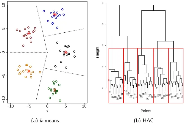
of easy implementation and good scalability. Figure 2.2a shows the cluster result
ob-tained by utilizing k-means upon a 2D dataset2 with the Euclidean distance function
(points labelled as∗in the figure are the centroids of the clusters). Other flat clustering
algorithms are based on the assumption that all the data are generated by some
mix-ture of underlying probability models (e.g., the Gaussian Mixmix-ture Model is commonly
used), so the clustering problem is transformed into a parameter estimation problem
where the parameters are determined by the underlying probability models. Then the
standard Expectation-Maximization (EM) approach can be applied: in the E-step the
cluster membership of all the data are identified and in the M-step the parameters of
the probabilistic models are optimized. Generally model-based clustering algorithms are
more mathematically understandable and reasonable than the proximity-based ones, but
care must be taken when choosing the functional form of the underlying probability
distributions.
Hierarchical clustering algorithms in contrast use a hierarchical structure to
or-ganize data, in which upper-level clusters contain the lower-level clusters. To generate
the hierarchy, we can either treat each data object as a separate cluster and then
grad-ually merge them in a bottom-up fashion, or start from a cluster containing all the data
objects and recursively divide the clusters in a top-down fashion. In addition to
calcu-lating the similarities between data objects, these algorithms require the definition of
similarity measure between clusters. The single-linkage and complete-linkage methods
are often used for hierarchy generation. Figure 2.2b shows the hierarchical structure
built by utilizing the hierarchical agglomerative clustering (HAC) algorithm upon the
1Medoid is the data object within a dataset of which the average distance to all the other objects in
the dataset is minimal.
same 2D dataset as in Figure 2.2a. Then an appropriate level in the hierarchy may
be selected as the cutting point to obtain a partitioning of the data (as the subtrees
surrounded by the red boxes in the Figure 2.2b).
Besides the above categorization, the clustering algorithms may also be
distin-guished as incremental or non-incremental, depending on whether or not they are able
to incrementally improve the cluster models when new data become available.
Addi-tionally, modern clustering algorithms can be categorized according to the techniques
they adopt, such as graph theory, spectral theory etc.
Propositional clustering algorithms are mainly proposed for analyzing datasets
in the multi-dimensional vector space, i.e. we have allxi ∈Rn in Definition 2.1. Based
on this assumption, many algebraic or geometric approaches can be utilized to facilitate
the calculation of the clustering procedure3. For example, BIRCH [162] adopted the
“Clustering Feature” (CF) to summarize the properties of a cluster, which is essentially
the linear sum and the squared sum of data vectors in the cluster. Other algebraic and
geometric features of the cluster such as the centroid, radius/diameter, the
intra-/inter-cluster distances can be computed from the CF vector. Moreover, the CF vector is easy
to be updated when new data are absorbed into the cluster.
However, many datasets in practice cannot be represented as multi-dimensional
numeric or nominal vectors. They are composed of heterogeneous data types and
inter-relationships. We refer to them as therelational datasets to emphasize their substantial
differences from the previouspropositional datasets. Obviously, the algebraic and
geo-metric theorems in the vector spaceRnare not necessarily correct in the relational data
space, for example the relational data instances are not additive or divisible as numeric
vectors. Naively applying propositional clustering algorithms cannot fully exploit
infor-mation contained in the dataset or leads to inappropriate conclusions about the data
[64], so analyzing relational datasets has become a critical challenge and an active
re-search direction in recent years. In the rest of this chapter, some fundamental concepts
3When processing a categorical dataset, we can use a different boolean dimension to represent each
Table 2.1: Propositional Iris Dataset
ID Sepal Sepal Petal Petal Class
(#) Length Width Length Width
1 5.1 3.5 1.4 0.2 Iris-setosa
2 4.9 3.0 1.4 0.2 Iris-setosa
3 4.7 3.2 1.3 0.2 Iris-setosa
. . .
51 7.0 3.2 4.7 1.4 Iris-versicolor
52 6.4 3.2 4.5 1.5 Iris-versicolor
53 6.9 3.1 4.9 1.5 Iris-versicolor
. . .
101 6.3 3.3 6.0 2.5 Iris-virginica
102 5.8 2.7 5.1 1.9 Iris-virginica
103 7.1 3.0 5.9 2.1 Iris-virginica
. . .
of relational clustering are introduced in Section 2.1 and then a state-of-the-art review
of relational clustering algorithms is provided in Section 2.2.
2.1
Fundamentals of Relational Clustering
As follows, Section 2.1.1 explains the properties of relational data and the methodology
of constructing relational data objects. Section 2.1.2 introduces a recursive similarity
measure to compare relational data objects. Section 2.1.3 provides some criteria to
evaluate the cluster quality.
2.1.1 Relational Data
Traditional data mining algorithms assume all data are represented as attribute-value
pairs. With such assumption, each data instance corresponds to a row (or tuple) in a
table and each attribute to a column [121]. In this paper, datasets that can be mapped
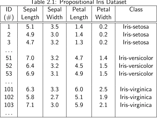
into a single table are called propositional. Table 2.1 is an example of propositional
dataset in the UCI Machine Learning Repository [7]. By analyzing these tuples, we can
Figure 2.3: Schema of a movie dataset
or Xiris−virginica = {x|0.6 < P etalW idth(x) ≤ 1.5 and P etalLength(x) > 4.9} ∪
{x|P etalW idth(x)>1.7}.
In contrast, relational datasets pertain to domains with different data types and
sets of relationships between them [36]. These data types together with the relationships
constitute a far more sophisticated feature space than those in propositional datasets.
According to the theory of relational database [28], a table stores a set of tuples with
the same attributes and a link between tables means that the referencing tuple has the
referenced tuple as part of its attributes, so we have:
Definition 2.2. A relational dataset contains a set of tables D = {X1, X2, . . . , XM}
and a set of relations (links, associations) between pairs of tables. All the tuples in the
tableXi are of the same type and tuples in different tablesXi andXj are semantically
associated by the relation(s) between Xi and Xj. To simplify our discussion, we use
Xi.c to denote the concept c of table Xi, where c might be an attribute in Xi or the
name of another table that is associated toXi.
Consider an example of a relational movie dataset, of which the schema is shown
in Figure 2.3. Each table contains a set of attributes to define an entity type (e.g.
Movie, Actor or Director) or a many-to-many relationship (e.g. director-Direct-movie
or actor-Act-movie). Links between tables indicate a one-to-many relationship (along
the direction of arrows). Based on this database schema, the original data instances
are decomposed before being stored in order to minimize the data redundancy. In the
such asjoin, we can easily retrieve all the information about an actor: his name and all
the movies he acted in as well as all the directors he worked with.
Because tuples in different tables of a relational dataset are semantically
as-sociated by the relationship(s) between these tables, Relational Patterns extends the
Propositional Patterns in the scenario of relational learning [76][121]:
Definition 2.3. Relational learning is “the study of machine learning and data min-ing within expressive knowledge representation formalisms encompassmin-ing relational or
first-order logic. It specifically targets learning problems involving multiple entities and
relationships amongst them.”
From the above definition, we can see that attribute values of tuples as well
as their pairwise linkage information are both important for relational learning. When
searching for patterns in a relational dataset, not only the tuples in the target table but
also those in the associated tables should be considered. Therefore, in the movie dataset
(Figure 2.3) the analysis of any actor should be based on the movies he has acted in
as well as the directors or other actors he cooperated with, so information stored in the
associated tables Movie and Director needs to be exploited. For example, a relational
pattern to strictly identify action movie stars can be described as X˜action = {x |x ∈
XActor,(x.movie).genre=Action}.
Sometimes propositional clustering algorithms are still applicable for processing
relational datasets by means of merging multiple tables into one (this operation is called
“propositionalization” [78]) , but it is not a good choice because [47][100]:
• Transforming relational linkage information as additional attributes in the target table often leads to a very high dimensional feature space. The derived tuples are
very sparse and thus inevitably degrades the performance of clustering algorithms.
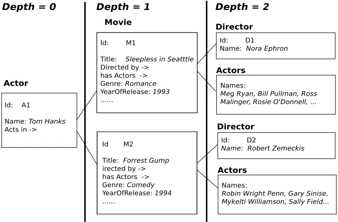
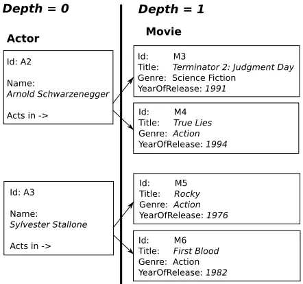
Figure 2.4: Example relational object for Tom Hanks
• The propositional clustering algorithms are originally designed for propositional datasets, and so they cannot capture the features that are propagated along the
paths of relationships between multiple data types.
The above limitations of applying propositional clustering algorithms to relational datasets
motivate the development of numerous relational clustering algorithms. As the basis of
further discussion, here we will first introduce an approach of constructing relational
data objects to systematically exploit the associated information for a target tuple.
Given a dataset schema represented as a directed graph G = (V, E), in which
vertices V = {ci} stand for the tables (concepts) in the schema and edges E =
{~est|edge~est : cs → ct; cs, ct ∈ V} for the relationships between concepts. An
edge~est : cs → ct means that the source concept cs references the target concept ct
as its associated feature. When constructing an objectx of conceptcs, we find out all
the associated featuresF(cs)and link any objecty of typect that satisfies the relation
Table 2.2: Properties of distance functions Distance Function Positivity f d(xi, xj)≥0
Reflexivity f d(xi, xj) = 0, iff xi=xj
Symmetry f d(xi, xj) =f d(xj, xi)
Triangle Inequality∗ f d(xi, xk)≤f d(xi, xj) +f d(xj, xk)
In the example of the data schema shown in Figure 2.3, according to the
rela-tionship structure, we haveF(Movie) ={Title,Genre,YearOfRelease,Duration,Actor,
Director} and F(Actor) = F(Director) = {Name, Movie}. Then all the associated
data objects are recursively linked to the current object. Figure 2.4 shows parts of the
relational data object constructed for Tom Hanks.
2.1.2 Proximity Measures
Many clustering algorithms as well as evaluation criteria are designed based on the
proximity (i.e. similarity or distance) values between pairs of data objects. Before
discussing the proximity measures for relational datasets, we first go through some
classic measures that are widely used in propositional datasets.
For any propositional dataset D = {x1, x2, . . . , xN}, we can either define a
similarity measure f s(·,·) or a distance measure f d(·,·). These measures have some
properties listed in Table 2.2 [35]. The property of triangle inequality is not necessary
for a proximity measure. When it is satisfied, the measure is also called a metric. It
is also worth noting that the distance measure f d(·,·) is generally unbound. In most
cases we can normalize the distance measure to limit its values within the interval[0,1].
Then the normalized distance measure can be converted into a similarity measure or
vice verse by utilizing the propertyf s(xi, xj) +f d(xi, xj) = 1.
The attributes of propositional data might be of typesnominal,numeric,
string-based, vector-based, etc. A variety of proximity measures are applicable for different
Table 2.3: Similarity Measure for Categorical dataset
α β Name of Similarity Measure 1 Jaccard Coefficient 0 2 Sokal and Sneath Measure
1/2 Gower and Legendre Measure 1 Simple Matching Coefficient 1 2 Rogers and Tanimoto Measure
1/2 Gower and Legendre Measure
• For nominal datasets, whenxi andxj denote single nominal values, a
straightfor-ward similarity function can be defined as:
f snominal(xi, xj) =
1 ifxi =xj
0 otherwise
(2.1)
In some cases, we expect to know the similarity between two sets of nominal values
ˆ
xi and xˆj. If we usen11 to represent the number of nominal values appearing in
both xˆi and xˆj, n00 for nominal values appearing in neither xˆi or xˆj, n10 (resp.
n01) for nominal values that appear in xˆi (resp. xˆj) only, a family of proximity
measures can be defined by [35]:
f s′nominal(ˆxi,xˆj) = n11+α·n00
n11+α·n00+β·(n01+n10)
(2.2)
Table 2.3 gives some possible combinations for parameters α and β, as well as
their corresponding measures.
• For numeric variables,xi andxj represent single values in the range (a, b) where
b > a. Then the distance can be calculated by:
f dnumeric(xi, xj) =
xi−xj
b−a (2.3)
oper-ations needed to transform one string into the other. Transformation operators
include insertion, deletion, or substitution of a single character. Then the
normal-ized distance function can be defined by:
f dstring(xi, xj) =
levenshtein distance(xi, xj)
string length(xi) +string length(xj)
(2.4)
• For two points in the n-dimension Euclidean space, Minkowski metric is widely used:
f dpoint(xi, xj) =
m
X
p=1
|xip−xjp|q
1/q
, q≥1 (2.5)
Settingq = 1 gives the Manhattan metric while q = 2is the familiar Euclidean
metric. When q → ∞, the metric converges to maxp|xip−xjp|.
• Whenxi andxj are numeric vectors, the cosine value of the angle between them
can be used as the similarity measure:
f svector(~xi, ~xj) =
P
pxip·xjp
qP
px2ip·
qP
px2jp
(2.6)
Such a model has been applied successfully in the fields of Information
Re-trieval(IR) and Collaborative Filtering(CF). Each index term of the document
or each user of the object is taken to be a orthogonal dimension in the vector
space, and so documents or objects are represented as weight vectors. In the IR
domain these weights can be obtained by TF-IDF ranking strategy [9], and in the
CF domain they are the ratings provided by users.
• In statistics, Correlation Coefficient refers to the departure of two random vari-ables x and y from independence: ρ = σxy
σxσy. If ρ = ±1, it means x and y are
maximally positively or maximally negatively correlated. Ifρ= 0, thenxandyare
surements have been developed, among whichPearson’s Correlation Coefficientis
the best known:
f sstat(xi, xj) =
P
p(xip−xi)(xjp−xj)
qP
p(xip−xi)2·qPp(xjp−xj)2
(2.7)
wherexi = 1
m
m
X
p=1
xip and xj = 1
m
m
X
p=1
xjp.
The propositional proximity measures introduced above are the foundation for
constructing the relational measures. Given two relational objects associated with
mul-tiple tables of different data types, we can first utilize some appropriate propositional
measures to compare their components and then synthesize the results as the total
prox-imity value for the objects. Horv´ath et al. proposed the RIBL2 measure in [60] : Given
two relational data objectsxi andxj of conceptcsconstructed as in Section 2.1.1, their
relational similarity is computed as:
f sobject(xi, xj) =
X
ct∈F(cs)
wst·f sset(xi.ct, xj.ct) (2.8)
where weight wst (wst ≤ 1 and Ptwst = 1) represent the importance of member
conceptctwhen describing the conceptcs. In Equation 2.8,f sset(xi.ct, xj.ct)is defined
as:
f s′set(xi.ct, xj.ct) =
1 |xi.ct|
X
yl∈xj.ct
max
yk∈xi.ct
f sobject(yk, yl), if|xi.ct| ≥ |xj.ct|>0.
1 |xj.ct|
X
yk∈xi.ct
max
yl∈xj.ct
f sobject(yk, yl), if|xj.ct| ≥ |xi.ct|>0.
0, if|xi.ct|= 0 or |xj.ct|= 0.
(2.9)
IfF(cj) 6=∅, the value off s(yk, yl) in Equation 2.9 is recursively calculated by
Equa-tion 2.8. This measure explores the linkage structure of the relaEqua-tional objects in a
Figure 2.5: Two Example Movie Stars
reached, where the propositional similarity metrics can be applied. Generally, the whole
linkage structure is not necessary to be exploited because the weightswst between the
referencing concept cs and the referenced concept ct make the impact of components
in low levels of linkage structure decreases exponentially.
Here is an example to demonstrate the above recursive similarity measure: in the
movie dataset we have F(Movie) = {Title,Genre,YearOfRelease,Actor,Director} and
F(Actor) = {Name,Movie}. Figure 2.5 shows the relational objects for action movie
stars “Arnold Schwarzenegger” and “Sylvester Stallone”. We compare them with the
actor “Tom Hanks” represented in Figure 2.4. In the scenario of propositional clustering,
actors are compared based on their names since no relational data are considered there.
If we regard the name of actors as a set of enumerated values and then utilize the
true-or-false function, the similarity between every pair of actors will always be zero because
they have different names. An alternative way is to use the Levenshtein distance to
compare the actors, then we have f s(oA2, oA3) = f sstring(“Arnold Schwarzenegger”,
“Sylvester Stallone”) = 0.095 and f s(oA1, oA3) = f sstring(“Tom Hanks”,“Sylvester
Table 2.4: Linkage Matrix between Actors and Movies
Name M1 M2 M3 M4 M5 M6
Tom Hanks (A1) 1 1 0 0 0 0
Arnold Schwarzenegger (A2) 0 0 1 1 0 0
Sylvester Stallone (A3) 0 0 0 0 1 1
Figure 2.6: Genre Taxonomy
If we transform the relational information into a high dimensional vector space,
e.g. constructing a binary vector to represent the movies that an actor has acted in,
the pairwise similarity between the actors can be calculated using the cosine value of
their movie vectors or simply using the equivalent Jaccard Coefficient. As shown in
Table 2.4, such a transformation will produce sparse data and hence bias the cluster
analysis. Another issue is that the semantic information about movie genres shown in
Figure 2.6 will be lost when calculating pairwise similarity between actors.
To illustrate the RIBL2 measure, we first calculate the similarity value between
movies “Terminator 2: Judgment Day” and “Rocky” (to simplify our calculation, the
weightswst for different associated concepts are set equally):
f sobject(oM3, oM5)
= 1 3 "
f sstring(oM3.T itle, oM5.T itle) +f staxonomy(oM3.Genre, oM5.Genre)
+f snumeric(oM3.Y ear, oM5.Y ear)
#
= 1 3
0.077 + 0.5 +
1− |1991−1976|
yearmax−yearmin
Similarly we have:
f sobject(oM4, oM5) =
1 3
0 + 1 +
1−|1994−1976| 30
= 0.467
f sobject(oM3, oM6) =
1 3
0.154 + 0.5 +
1−|1991−1982|
30
= 0.451
f sobject(oM4, oM6) =
1 3
0.182 + 1 +
1− |1994−1982| 30
= 0.594
Based on the above similarity values between movies, we can calculate the similarities
between actors as follows:
f sobject(oA2, oA3)
= 1 2 h
f sstring(oA2.N ame, oA3.N ame) +f sset(oA2.M ovie, oA3.M ovie)
i
= 1 2
0.095 + 1 2
X
yl∈{M5, M6}
max
yk∈{M3, M4}f sobject(yk, yl)
= 1 2
0.095 +1
2(0.467 + 0.594)
= 0.313
In the same way, we can get f sobject(oA1, oA3) = 0.171 < f sobject(oA2, oA3), which
means Sylvester Stallone (A3) is more similar to Arnold Schwarzenegger (A2) than
Tom Hanks (A1). Therefore, by utilizing the relational proximity measure to exploit the
linkage structure within the relational dataset, we achieve more credible results about
the object comparison.
The idea of mutual reinforcement has also been utilized recently to iteratively
calculate similarity values between relational data objects. Jeh and Widom [63]
stud-ied the structural-context similarity of relational data objects. Their similarity measure,
namedSimRank, is based on the principle “two objects are similar if they are related to
similar objects”. Given the original relational objects represented as a usual graph G,
they construct an ordered node-pair graph G2 in which each node represents a pair of
an iterative fixed-point algorithm is used to compute the SimRank scores for the
node-pairs in G2. The authors proved in theory that the solution for the SimRank equation
is existent and unique. They also showed that their SimRank model is mathematically
equivalent to the expected-f meeting distance in a random surfer-pairs model. Fogaras
and R´acz [44] improved the scalability of the original SimRank approach by
introduc-ing the idea of randomized Monte Carlo methods combined with indexintroduc-ing techniques.
Xi et al. [154] proposed a Unified Relationship Matrix (URM) to represent a set of
heterogeneous data objects as well as their interrelationships. Based on that, they
de-veloped a unified similarity-calculating algorithm, SimFusion, by iteratively computing
over the URM until reaching the convergence. The theoretical analysis showed that
the URM can be considered as a single step transition matrix of a Markov Chain and
the iterative similarity reinforcement process of updating the Unified Similarity Matrix
is equivalent to a “two random walker model”. Although the effectiveness of SimRank
and SimFusion are supported by some experimental results, their computational
com-plexities are quadratic with respect to the number of data objects. Xue et al. [156]
developed a Multiple Relationship Similarity Spreading Algorithm (MRSSA) to compute
similarities for multiple object types in an iterative spreading fashion. They first use
a graph-based model to represent the linkage structure within a relational dataset and
define the relational similarity measure as a linear combination of the content similarity
as well as the and inter-type similarities between data objects. Because the
intra-and the inter-type similarity mutually affect each other, an iterative process is used to
improve the precision of pairwise similarities between data objects. White and Smyth
[148] define and evaluate a host of metrics to compute the similarity between a given
object and the other reference objects in a graph. The above reviewed measures do not
always satisfy the property of Triangle Inequality in Table 2.2, which means they are not
metrics. To address this issue, some relational distance metrics like [123] or [122] have
2.1.3 Evaluation Criteria
In this section we consider another important question: If the proximity measure has
been chosen, which criterion should be used to guide the cluster analysis and evaluate
the derived results? Clustering can be regarded as a search problem with each node
corresponding to a certain partitioning [112], but exhaustively evaluating all possible
partitions to find the optimal one is infeasible in practice due to the high computational
complexity. Therefore some heuristic methods are utilized in the design of clustering
algorithms to accelerate the search. It has been pointed out that the procedure of cluster
analysis is considerably subjective in nature: the target data objects are partitioned into
“a number of more or less homogeneous subgroups on the basis of an often subjectively
chosen measure of similarity (i.e., chosen subjectively based on its ability to create
interesting clusters)” [8]. Hence, the evaluation criterion plays an important role for
the cluster analysis. It guides the search direction in the partitioning space as well as
quantitatively evaluating different partitions derived by clustering algorithms to find the
optimal one.
Some criteria for propositional datasets are outlined in [35]. Among whichSum
of Squared Error (SSE) is the most widely used for clustering. LetK be the number of
derived clusters,Nk be the number of data instances in clusterCkandxkbe the center
of these data. The SSE criterion is defined as:
E=
K
X
k=1
X
x∈Ck
f d2(x, xk) (2.10)
The SSE criterion is appropriate when the clusters are compact and well separated
from each other. However, when the number of data objects in the optimal partition
vary greatly, the cluster result with minimum SSE may not reveal the true underlying
data structure, because a partition splitting large clusters is more favorable under such
circumstance. It means those clustering algorithms designed based on the principle of
size. To address this issue, another criterion,Related Minimum Variance, might be used:
E= 1
2
K
X
k=1
Nksk (2.11)
where
sk=
1
N2
k
X
x∈Ck
X
x′∈C
k
f s(x, x′) or sk= min x,x∈Ck
f s(x, x′)
The SSE or Related Minimum Variance criterion can be applied in the functionsFintra(Ck)
andFinter(Ck, Ck′) of Definition 2.1 to guide the clustering procedure or evaluate the
derived result. For example, ink-means we iteratively adjust the membership of data
instances in each cluster in order to reduce the SSE value over all the clusters.
The SSE criterion, also named as theWithin-cluster Scatter Matrix (denoted as
SW) in multiple discriminant analysis, can be used to evaluate the intra-cluster distances.
Additionally, the criteria of Between-Cluster Scatter Matrix and Total Scatter Matrix
(denoted asSB andST respectively) are used to evaluate the inter-cluster distances and
the scattering extent of the whole dataset respectively:
SB =
K
X
k=1
Nk·f d2(xk, x) and ST =
X
x∈D
f d2(x, x) (2.12)
where xk is the center for all data objects in cluster Ck as before, x is the center for
the whole dataset. In propositional clustering, the center of a cluster is the mean of all
data in that cluster: xk = N1kPx∈Ckx when clusterCk⊂R
m. Similarly we have x=
1
N
P
x∈Dx. However, in relational clustering the center of a cluster is usually determined by the medoid of all data objects in that cluster, so the constraintST =SW+SB that
is valid in propositional datasets will be invalid for relational clustering. Additionally,
the operation of determining the medoid within a cluster has quadratic computational
complexity. Such disadvantage heavily restricts the application of relational clustering
algorithms that are designed to minimize the SSE criterion of a partition for a relational
To evaluate the quality of the cluster result, it is possible to examine the
homo-geneity within the clusters and the heterohomo-geneity between the clusters when the class
labels of data objects are available. The Jaccard Coefficient [141] is suitable for this
purpose, which is computed by the number of pairs of objects in same cluster and with
same class label over that of pairs of objects either in same cluster or with same class
label. In Table 2.3 we set the parametersb= 0andw= 1to get the Jaccard Coefficient.
Alternatively, we can evaluate the quality of clusters based on the idea of entropy.
Entropy was first introduced in thermodynamics to measure the system’s thermal energy.
Being obtained from the disordered molecular motion, entropy reflects the molecular
disorder in the thermodynamic system [51]. Later, entropy was extended to measure
the uncertainty associated with a random variable in information theory [133]. Recently
the entropy is used to evaluate the disorder or impurity of clusters [145]. Formally, given
the class labels of data objects in a clusterCk,Ck’s entropy is computed by:
E(Ck) =−
X
h
Ph,klog2Ph,k (2.13)
where Ph,k is the proportion of data objects of class h in the cluster Ck. The total
entropy is defined as:
E =X
Ck
E(Ck) (2.14)
Generally speaking, smaller entropy values indicate higher accuracy of cluster result.
2.1.4 Determining the Number of Clusters
In this section we will briefly discuss another issue in clustering: how to determine an
appropriate number of clusters that should be generated? Obviously the quality of final
cluster result is heavily dependent on such number: too many derived clusters will break
linkages between similar data instances and thus cause the loss of pattern information;
while too few derived clusters will hide the pattern within noise and make the result
clusters as an input parameter and in most cases such number has to be estimated based
on background knowledge or exclusive analysis on the dataset itself. So determining the
number of clusters is considered as “the fundamental problem in cluster validity” [34].
Xu and Wunsch summarized four approaches in [155] to estimate the appropriate
number of clusters for propositional clustering algorithms:
• Visualizing datasets: When the dataset can be mapped to points in a 2D or 3D space, we will use some graphical tools to visualize the distribution of data
instances and thus estimate the optimal number of clusters. However, the
appli-cability of this approach is restricted because of the complexity data structure in
most real dataset.
• Constructing certain indices (stopping rules): These indices are generally based on evaluating the compactness of derived clusters, e.g. the squared error, the
intra-cluster similarity and inter-cluster distance or some synthesized criteria, to
determine the optimal value ofK. One disadvantage is that the success of these
indices is data dependent, which means the good performance of an index upon
one dataset does not guarantee it works well on other datasets [41].
• Optimizing some criterion function under probabilistic mixture-model framework; The clustering problem can also be solved using EM algorithm, i.e. using data
to estimate parameters of probabilistic models for a given range of K and then
select the optimal K that maximize some predefined criterion. Many criteria
based on various ideas in statistics, Bayesian theory or information theory have
been proposed [150][117][115].
• Utilizing other heuristic approaches: For example, eigenvalue decomposition on the kernel matrix in the feature space has been investigated to determineK [49].
Ideally we expect the clustering algorithms can automatically adjust the number of
clustering the above goal has been achieved more or less by utilizing the above
ap-proaches. However, in relational clustering the problem is more sophisticated because
cluster results of different data types are inter-related, which means skewed clusters of
one type caused by an inappropriate K will propagate along the linkage structure to
influence partition of other data types and thus deteriorate the global cluster results.
To the best of our knowledge, there are no systematic studies on how to determine the
optimal number of clusters in relational cluster analysis.
2.2
Relational Clustering Algorithms
Relational clustering algorithms can be categorized as proximity-based, reinforcement,
model-based, graph theoretic and constraint-based approaches. Among them the
rein-forcement clustering is the only one not rooted in propositional clustering approaches.
We now discuss each of these categories in turn.
2.2.1 Proximity-based Clustering
As discussed in the previous section, proximity-based approaches can be distinguished
as flat clustering and hierarchical clustering.
Flat clustering approaches assign data into a set of disjoint clusters without
hi-erarchical relationship between each other. Since finding the global optima is usually
infeasible in practice, some heuristic techniques are incorporated to accelerate the
pro-cedure. Based on the proximity measures introduced in Section 2.1.2, the clustering
procedure begins at a random partition and then approximates the optimal solution by
minimizing a specific criterion (Section 2.1.3) in each iteration. When the error falls
under an acceptable threshold or the assignment of data to the clusters no longer change
from one iteration to another, which is regarded as “convergence”, the partition will be
output as the final result. The most well-known partitional clustering algorithms are
global search and faster convergence (e.g. genetick-means algorithm (GKA) [79] and
globalk-means algorithm [95]), to find arbitrary cluster shapes (e.g. DBSCAN [39] and
OPTICS [5]), etc.
Hierarchical clustering approaches organize all data using a hierarchical structure,
called a “dendrogram”. The root node represents the whole dataset and each leaf node
is regarded as a data object. Each intermediate node in the dendrogram corresponds
to a subset of the dataset, in which the data are grouped according to their pairwise
proximity. The ultimate cluster result is obtained by cutting the dendrogram at an
appropriate level. Hierarchical clustering approaches can be performed divisively or
agglomeratively. The former methods start by assuming the entire dataset belongs to
the same cluster and successively divides it into sub-clusters. The agglomerative methods
begin with each data object in a distinct (singleton) cluster and successively merges them
together. Various linkage criteria, for example single-linkage, complete linkage, average
linkage, median/centroid linkage or Ward’s method [155], can be used to compute the
pairwise proximity between clusters. The common disadvantages of classic hierarchical
clustering approaches include the high computational complexity and the sensitivity to
outlier data. Hence, new algorithms such as BIRCH [162], CURE [52] and Chameleon
[68] were developed to address these issues.
Since the flat and the hierarchical clustering approaches are both based on
prox-imity measures, they might be extended to process relational datasets by incorporating
the relational proximity measure introduced in Section 2.1.2. Kirten and Wrobel
de-veloped RDBC [72] and FORC [71] as the extensions of propositional hierarchical
ag-glomerative andk-partitional algorithms respectively. Both of them adopt the measure
RIBL2 [73] to evaluate the distance between data objects. However, since objects in the
relational dataset are normally not additive or divisible as numeric vectors, RDBC and
FORC have to use the medoids to represent the center of clusters instead of using the
means. The medoid of a cluster is defined as the data object that has the maximum
clus-ter. To achieve this, all pairs of data objects in the given cluster have to be compared.
Therefore, RDBC and FORC are not suitable for clustering very large datasets as they
have quadratic time complexity.
2.2.2 Reinforcement Clustering
The principal of reinforcement clustering approaches comes from the observation that,
since all data objects of different types are inter-related to each other, the cluster result
of one data type might be propagated along the relationship structure to improve that of
other data types. Anthony and desJardins summarized this idea asinter-cluster relation
signature [6]: First, data objects of a certain type, assume ci, are clustered based on
their attributes using some propositional clustering methods; Then for other objects of
type cj referencing (or being referenced by) ci, the inter-cluster relation signature is
constructed as a K-dimensional vector, whereK is the number of clusters obtained in
the first step. The value of each dimension in the inter-cluster relation vectorvk is the
number of edges that an object of type cj has when being linked to objects of type ci
in clusterk. Hence, the data objects of type cj are clustered based on the above
inter-cluster relation vector in addition to their propositional attributes. The above iterative
procedure continues until the clusters of all data types become stable.
The relational clustering algorithm motivated by the idea of mutual reinforcement
was firstly implemented by Zeng et al. [160] in the scenario of clustering heterogeneous
web objects, such as web-pages/users or queries/documents. They analyzed several
cases of mutual reinforcement in clustering, and concluded that “when the links among
nodes are dense enough and contain mostly correct information”, the cluster results of
one data type will improve that of other related data types. Additionally, they use a
hybrid similarity function, a weighted sum of two similarity measures based on content
features and link features, to compare data objects during the clustering procedure.
The ReCoM framework proposed by Wang et al. [145] further developed this idea by
being used to group data objects in an iterative reinforcement fashion, the relationship
structure is also used to differentiate the importance of data objects. More important
objects, just as authoritative and hub nodes as produced by the HITS algorithm [75],
can have more influence on the clustering procedure. When clustering data objects of a
certain type, both of the above frameworks will transform the information of relationship
structure into the link feature vector of the current objects according to the cluster result
of other data types. By this means, the relational clustering task is propositionalized
and thus propositional clustering algorithms could be easily embedded into each iterative
clustering step to improve the efficiency.
Yin et al. [157] proposed another relational clustering approach, LinkClus, which
is also performed by using reinforcement. Instead of using the numeric vectors to
rep-resent the content and linkage features of relational objects, in LinkClus they designed
a hierarchical data structureSimTree to simplify the calculation of similarities between
objects, and then use LinkClus to improve the SimTree iteratively. One drawback in
LinkClus is that they only utilized frequent pattern mining techniques to build the initial
SimTrees and use path-based similarity in one SimTree to adjust the similarity values
and structures of other SimTrees, so information contained in the property attributes
of data objects are not used in their clustering framework. Ignoring such information
would definitely degrade the accuracy of the final clustering result.
2.2.3 Model-based Clustering
From the viewpoint of probability theory, data objects are assumed to be generated by a
set of parametric probability models. The derived clusters, which are expected to reflect
the natural structures hidden in the dataset, should match the underlying models. These
probability distributions might be of different types or have the same density function but
with different parameters. If the distributions are known, finding clusters within a given
data set is equivalent to the problem of estimating parameters for underlying models.