The accuracy and information content of two traditional statistical methods in forecasting bankruptcy: evidence from European countries

(1)

The accuracy and information content of two traditional

statistical methods in forecasting bankruptcy: evidence from

European countries

MSc thesis in the area of Business Administration Name: Bas Machielsen

Student no.: s1131044

University: University of Twente

Faculty: School of Management and Governance Supervisors: Prof. dr. R. Kabir

(2)

ii

iv Abstract: This study encompasses a treatment of underlying theory and specifications of various bankruptcy prediction models. It assesses the accuracy and information content of some of these models for publicly listed firms in the European Union. The models used to forecast bankruptcy include Altman (1968)’s Z-score model and the logistic regression model by Ohlson (1980). It is investigated what predictors are best, whether the model performance declines over time and which model does the best job of forecasting bankruptcies. The performance is assessed in an estimation sample (2005-2007) and in a hold-out sample (2011-2013). Model performance is evaluated alongside several criteria. It is found that both models lose a significant amount of predictive accuracy when applied out-of-sample, but they still carry information content. Many tests show that a significant amount of information is left uncaptured by the models. This generalizes through various sets of predictors. The findings are subjected to several benchmarks and robustness tests.

(5)

v

ACKNOWLEDGEMENTS

This Master Thesis came to be as a final result required for obtaining the degree of Master of Science in Business Administration at the University of Twente, Enschede, The Netherlands.

I would like to express my gratitude towards, and admiration for the scientific guidance of my two supervisors, prof. dr. Rezaul Kabir and dr. Xiaohong Huang, both of whom offered much

worthwhile advice and suggestions to substantially improve my research.

Finally, I would like to thank my family and friends for their interest, support and patience.

Of course, all errors and mistakes remain solely the responsibility of the author.

Bas Machielsen,

(6)

1

1. Introduction

The topic of bankruptcy prediction is a long standing topic in academia and has been extensively researched since the inception of Altman’s Z-score model (see Altman, 1968). Since then, several models have been developed and used in practice to predict bankruptcy. In recent years, especially during the ongoing economic crisis, increased attention has been paid to bankruptcy prediction models. The main problem that will be addressed in this study is to what extent two commonly-used statistical models are able to predict corporate bankruptcy. The central research question is ‘what is the accuracy and information content of two

statistical models predicting bankruptcy for a sample of listed non-financial European firms?’

In the scientific literature, bankruptcy prediction models are usually divided into statistical bankruptcy prediction models, and non-statistical bankruptcy prediction models (see Kumar and Ravi, 2007). In this study, the focus lies on statistical models because by far the largest body of bankruptcy forecasting features statistical models (see Bellovary et al., 2007, Westgaard, 2007). However, it will also feature reviews of non-statistical bankruptcy

prediction models, such as intelligent models, and some miscellaneous models. The research design is based predominantly on a combination of the methods of Altman (1968) and Ohlson (1980) but will feature some minor elements proposed and developed by, among others, Shumway (2001), Wu, Gaunt and Grey (2010) and Bauer and Agarwal (2014). The performance of these models is evaluated by assessing both in-sample and out-of-sample accuracy and information content. Accuracy serves as a metric for how many firms in the sample a model can predict correctly. Information content measures whether one model score contains more information about bankruptcy than another variable (or set of variables). The latter is assessed by means of the hazard modeling approach of Shumway (2001), employed by e.g. Chava and Jarrow (2004), Campbell et al., (2008) and in a slightly different way by Wu, Gaunt and Gray (2010) and Bauer and Agarwal (2014). Thus, it builds on various research designs commonly used in academia to forecast bankruptcy.

(7)

2 Among the interest groups in the prediction of financial distress or bankruptcy are creditors, auditors, stockholders and senior management, and employees of a firm (Kumar and Ravi, 2007, Bauer and Agarwal, 2014). Financial distress or eventually bankruptcy would affect them all alike. Bankruptcy prediction can also be used to assess the probability of bankruptcy that takes into account characteristics of specific sub-populations (e.g. SME's, private

companies, listed companies, companies in the manufacturing industry, etc.), tuned to

changes in the macro environment. Taking recent developments into account (i.e. the financial crisis of 2008, the debt crisis of 2010, implementation of Basel-III and the recession across Europe), the importance of scrutinizing banks and corporations has arguably become even more interesting and urgent for policy makers as well as for the general public.

Up until now there have been different, contradictory empirical results concerning the best-performing models and their inputs (compare e.g. the results of Hillegeist et al., 2004, Agarwal and Taffler, 2008, Trujillo-Ponce et al., 2013, Bauer and Agarwal, 2014). Research that compared one bankruptcy prediction model against another, often conflated evaluating the performance of particular sets of predictor variables with evaluating the performance of the econometric model (e.g. Grice and Dugan, 2003), violating a ceteris paribus clause. The literature in the past often evaluated the performance on a rather limited basis, i.e. either the accuracy or the information content, but not both. In most cases, there is also a lack of a proper benchmark with which the results are compared to. This research aims to evaluate model performance on the basis of multiple criteria and subjects the findings to several robustness tests. Furthermore, there is not much empirical research about model validity during the recent financial crisis. This research attempts to follow the line of Mensah (1984) and Begley et al. (1996) by addressing the problem of whether the model accuracy and information content change under changing macroeconomic circumstances, as changing circumstances can impact the stationarity of predictor variables as well as firm-invariant default risk. In this study, the events after credit crisis of 2007 and the subsequent European debt crisis of 2010 represent these changed circumstances.

The foremost contribution of this study is that it provides an empirical test in a cross-European context in two periods of different macroeconomic circumstances (i.e. the 2004-2007 and 2010-2013 period). Consequently, it provides for rigorous model robustness tests (cf. Grice and Ingram, 2001, Grice and Dugan, 2003), because if the models capture essential information about bankruptcy, model performance should remain stable over time, and the model should not only be expected to work in a country-specific context, but also in a cross-country context. Furthermore, existing empirical research predominantly focuses on U.S. (e.g. Altman, 1968, Ohlson, 1980, Shumway, 2001, Hillegeist et al., 2004) or UK (Agarwal and Taffler, 2007, 2008, Bauer and Agarwal, 2014) listed firms – except for one study, no

(8)

3 focused on predictive accuracy (e.g. Altman, 1968, Ohlson, 1980 but also Begley, Ming and Watts, 1996) or information content (e.g. Hillegeist et al, 2004). Finally, this study features many sets of predictor variables. Practitioners who have an interest in good bankruptcy prediction models might find it useful to see which set of variables performs best. From a scientific point of view, this is an investigation of whether model performance is sensitive to different sets of predictor variables.

This thesis is structured as follows: in chapter two, I present the theory underlying the

(9)

4

2. Literature review

In this chapter, a systematic overview of the development of and improvements on

bankruptcy prediction models used in academia will be given. Following Kumar and Ravi (2007), I make a distinction between research utilizing statistical bankruptcy prediction models, and research utilizing so called intelligent bankruptcy prediction models, including, among others, research utilizing neural networks, case-based reasoning and decision trees (Kumar and Ravi, 2007). The main focus will be on the statistical techniques, but the review will feature a comprehensive review of several intelligent techniques. The literature review seeks to explain the various methodologies and models utilized, to accentuate similarities and differences, and offer a systematic history of the introduction and methodological

development of various models.

First, the focus will be on research using statistical techniques. Each technique will be treated extensively, followed by some general critique and limitations. Second, a section will be devoted to the different ways of evaluating the accuracy of such a model, and the different ways the models have been evaluated in the past. Third, a short, comprehensive section will treat the evaluation of the information content of a model and what is meant by information content. Fourth, a brief statement about the evaluation of the economic value of a model will be provided. Furthermore, in treating each model separately, this review seeks to give a comprehensive account of the empirical results yielded. The empirics sections will feature a short comparison between the empirical results yielded by statistical models with the

empirical results yielded by intelligent techniques and the implications for future research. Finally, a summary table containing the most important contributions and findings, sorted by methodology, will be provided and the implications of recent research will be discussed.

2.1 Statistical bankruptcy prediction models

Similar to Bauer and Agarwal (2014), I propose to conceptualize the research focusing on statistical techniques into four different categories with regards to the kind of methodology (estimation procedure) used: (i) discriminant analysis models (e.g. Altman, 1968, Deakin, 1972, Grice and Ingram, 2001), (ii) logistic regression and similar models (Martin, 1977, Ohlson, 1980, Zmijewski, 1984), (iii) Distance-to-default models (e.g. Vassalou and Xing, 2004, Hillegeist et al., 2004, Shumway & Bharath, 2008), and (iv) hazard models (e.g. Shumway, 2001, Chava and Jarrow, 2004).

In treating the empirics of the models, I will accentuate differences between accounting-based and market-based predictors, because there is disagreement over whether any of these models should incorporate accounting-based information, market-based information, or both. Sloan (1996) argues that accounting data can be used to complement market data, since market prices are not an indication of company accounts in the present, but rather a prospect in the future.

(10)

5 Also, accounting numbers can be manipulated by the management. Nowadays, common practice is combining accounting and market data, for example in simple discrete time logit models following Shumway (2001). Chava and Jarrow (2004) use a mixture of accounting and market-based ratios consisting of profitability, liquidity as well as market volatility or market price. Campbell et al. (2008) use both accounting and market information by using ratios that contain both accounting and market data into one ratio.

In other words, there is no strict separation of accounting and market data anymore, and most research incorporates the informational benefit of both. Whether it is actually useful to do so, (i.e. whether it improves accuracy or information content) is however an empirical matter and will be discussed.

2.1.1 Discriminant analysis

Since the research of Altman (1968), prediction of financial distress and bankruptcy has incorporated statistical techniques instead of less systematic assessments. In prior research, academics (e.g. Beaver, 1966, 1968) tended towards ratio analysis in assessing and predicting financial distress in particular companies. The research was practically limited to comparing different accounting ratios of different firms in order to assess the degree of financial distress companies were in. Altman (1968) proposed a sound methodology, utilizing multivariate discriminant analysis (MDA) in order to provide a mathematically sound way to forecast financial distress, thereby starting a series of research which provides a rigorous framework of bankruptcy prediction utilizing various statistical techniques.

The purpose of the study of Altman (1968) is to attempt an assessment of the quality of ratio analysis as an analytical technique. The research improves on previous work which

“compared a list of ratios individually for failed firms and a matched sample of non-failed firms. Observed evidence for five years prior to failure was cited as conclusive that ratio analysis can be useful in the prediction of failure.” The poverty of sole ratio analysis without further data treatment was that “the methodology was essentially univariate in nature and emphasis was placed on individual signals of impending problems.”

MDA was used because it classifies “an observation into one of several a priori groupings dependent upon the observation's individual characteristics (Altman, 1968).” This

methodology fits the problem because the problem is classifying firms into either the

‘bankrupt’ class or the ‘non-bankrupt’ class, making use of some available financing ratios for each individual firm. MDA then derives from the data a linear combination (in this case of financial ratios) which discriminates best between both classes (in this case bankrupt or non-bankrupt).

2.1.1.1 Model description

In general, discriminant analysis combines an n number of independent variables into a linear function that discriminates best between two classes, i.e. such that the outcome of this

(11)

6

! = #_$%_$+ #₍%₍+ ⋯ + #_*%_*+ + Eq. (2.1)

where v1, v2, … vn= discriminant coefficients (weights) attached to x1, x2, … xn= independent

variables. The discriminant variate Z is the linear combination of independent variables that will discriminate best between the objects in the groups defined a priori. The function thus transforms individual variables to a single discriminant score or Z-value which is then used to classify the object firm. v1… vnare determined such that the separation S between the two

distributions (i.e. bankrupt and non-bankrupt) is as large as possible and accordingly that the discriminating ability is maximized.

Discriminant analysis is the appropriate technique for testing the hypothesis that the group means of a set of independent variables for two or more groups are equal. The test for statistical significance of the discriminant function is a generalized measure of the distance between so-called centroids. The centroid is defined as the arithmetic mean discriminant score of a class. Multiple discriminant analysis is unique in one characteristic compared to generic multivariate regression analysis: discriminant analysis is applied when the binary dependent variable is categorical, rather than ratio or interval. A mathematical treatment of the

estimation produce can be found in appendix A.

Altman (1968) notes that “the primary advantage of MDA in dealing with classification problems [in comparison with ratio analysis] is the potential of analyzing the entire variable profile of the object simultaneously rather than sequentially examining its individual

characteristics.” MDA is utilized to establish a function which best discriminates between elements in two mutually exclusive groups: in our case, bankrupt and non-bankrupt firms. Z-scores are not explanatory theories of failure (or success) but pattern recognition devices.

2.1.1.2 Model assumptions

The most prominent assumption underlying discriminant analysis is multivariate normality. Multivariate normality is a generalization of the univariate normal distribution to higher dimensions. This means that the used set of (possibly) correlated real-valued predictors should cluster around a mean value. Multivariate normality is not easily tested for, but standard practice is to test for univariate normality using the Shapiro-Wilk test (see Lo, 1986, Hair et al., 2006). Nevertheless, in practice, violation of these tests is ignored because “a rejection of normality on the basis of such tests does not leave the econometrician with a clear alternate method of analysis (Lo, 1986).”

(12)

7 strict assumptions have made for extensive critique (Ohlson, 1980, Zmijewski, 1984, among others) on the usage and usefulness of discriminant analysis in predicting bankruptcy. In the case of bankruptcy prediction, the most restrictive assumption is probably the assumption regarding independent observations: most research has been conducted within one particular country. In the case of research encompassing multiple countries, nonrandom sampling might lead to biased estimates towards ‘median’ countries. The discriminating ability of the model appears to be sensitive to outliers. It would also seem doubtful whether financial ratios are in fact normally distributed.

The fact that Altman’s bankruptcy prediction model is still used throughout academia leads to the question whether Altman's original model is as useful for predicting bankruptcy in recent periods as it was for the periods in which it was developed and tested by Altman. The

assumption in using the model with the same coefficient estimates in a hold-out sample is that the model is robust across (macro) economic conditions that change over time, such as

inflation, interest rates, and credit availability (see Nam et al., 2008, Tinoco and Wilson, 2013) and predictor variables must remain stationary. The effect of changing economic factors on the accuracy, magnitude, and significance of model coefficients was evaluated by Mensah (1984), Begley, Ming and Watts (1996) and Grice and Ingram (2001) and all of them reported that the accuracy and structure of the models changed over time.

In practice, researchers report that these assumptions of discriminant analysis are often violated (e.g. Altman, 1968, Altman and McGouch, 1974, Ohlson, 1980, Mensah, 1984). It should be noted that the key is, however, to build an empirically sound model, despite

relatively minor theoretical objections. Indeed, much research (e.g. Hillegeist et al, 2004, Wu, Gaunt and Gray, 2010) uses discriminant analysis as a benchmark model, regardless of

whether the assumptions are met. Sometimes, these models generally do indeed yield good results (for recent examples, see e.g. Agarwal and Taffler, 2007, 2008) despite the violations of the aforementioned assumptions.

2.1.1.3 Model empirics

In this section I will briefly go through the empirical research that utilizes the

MDA-methodology and will look for implications for further research. I will first treat articles that contain static tests of the MDA-methodology. This means that the emphasis of this research lies on model performance at one point in time, and not in the model performance over time. Afterwards, I will treat dynamic tests, i.e., research explicitly focusing on model performance over time.

Static tests: Discriminant analysis was developed as a multivariate improvement of assessing the quality of ratio analysis in the prediction of bankruptcy as executed in Beaver (1966). Beaver (1966) investigated industrial firms from the Moody’s Industrial Manual database. He compared means between bankrupt and non-bankrupt firms, subjected the findings to

(13)

8 The study of Altman (1968) features the first application of discriminant analysis to

bankruptcy prediction. He investigates a U.S. manufacturing sample of 100 bankrupt and 100 non-bankrupt firms and reports that the discriminant analysis model is extremely accurate in classifying 95 per cent of the total sample correctly. In two years before the occurrence of bankruptcy, 72 per cent correct assignment is evidence that bankruptcy can still be predicted two years prior to the event. The errors do increase when the period to bankruptcy increases, so after two years the model cannot significantly distinguish bankrupt from non-bankrupt firms anymore.

Deakin (1972) emulates the research methodology by Altman (1968). He selected 11 failed and 23 non-failed firms at random from the Moody’s Industrial manual. He indicated that misclassification errors averaged 3%, 4.5%, and 4.5% for the first, second and third years respectively. He also noted that incorrect classification as failed (type II errors) happens more often than incorrect classification as non-failed (type I errors). The accuracy of the

discriminant analysis model declines when applied 4 or 5 years before the occurrence. This is in line with the results of Altman (1968), although Deakin’s (1972) results show slightly greater robustness over time.

Begley et al. (1996) applied discriminant analysis and logistic regression (see 2.1.2) models to prediction bankruptcy for 1365 industrial firms, which is a broader application than used by Altman, who conducted his research on a sample of manufacturing firms. They used data from the S&P COMPUSTAT database. The models performed relatively well when they were estimated, but they find that they do not perform as well in more recent periods, even after re-estimation of the coefficients. The original logistic regression model displays the strongest overall performance. These results are important because they suggest other variables might predict bankruptcy better than the ones chosen by Altman (1968).

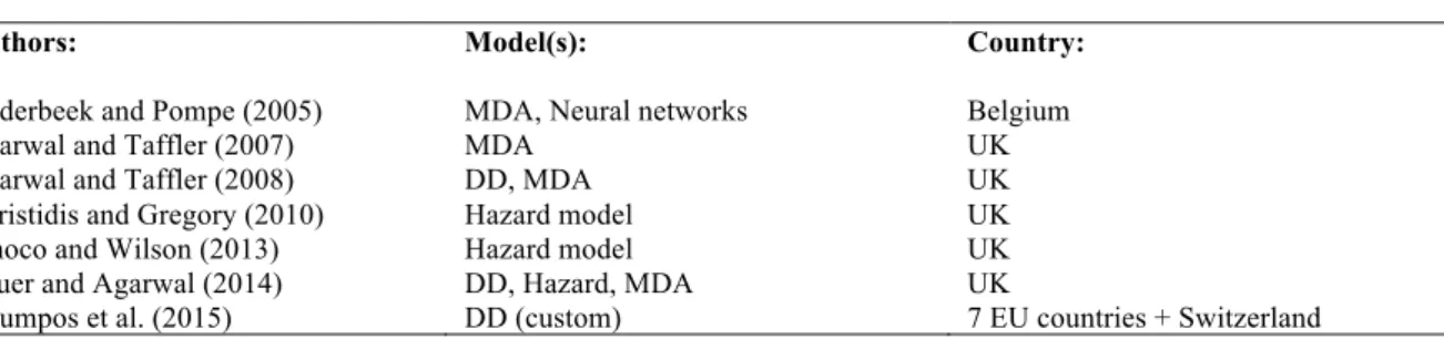
Pompe and Bilderbeek (2005) applied discriminant analysis and neural networks (see section 2.2) to the problem of bankruptcy prediction. Both methods produced similar results. They use factor analysis to determine the ratios included in the prediction models, and evaluate by means of classification tables (see section 2.3). Their sample included Belgian SME’s from 1986 until 1994. Their data comes from the Belgian National Bank. The results showed that almost every ratio they had considered showed predictive power. Thus, an approaching bankruptcy is noticeable in almost every dimension of a firm's financial position. A few ratios, such as cash flow/total debt, achieved results that were close to the results of complete sets of other ratios. They also investigated the stationarity of their selected variables (i.e. constant mean, variance and covariance over time); it was found that the predictive power of the models were not sensitive to nonstationary variables.

(14)

9 recalibration of the model coefficients accordingly leads to superior accuracy. This implies that the model should be re-estimated in every period of time and that the model is generally not robust to changes in the macroeconomic environment. Thus, these results contradict Deakin’s (1972) and Altman’s (1968) earlier results of a significant model robustness and stable coefficients over time. They imply that such research designs introduce a bias.

Mossman et al. (1998) investigate a sample of U.S. non-financial firms. Their accounting-based data ranges from 1980-1991 and comes from Compustat and their market data from CRSP. They test four sets of predictor variables: so-called ratio models, cash flow models, return models and return variation models. These ratios then serves as input in either a logistic regression based on Ohlson (1980) or a MDA model based on Altman (1968) Based on a sample of bankruptcies from 1980 to 1991, results indicate that no existing model of

bankruptcy captures the data completely: “the discriminatory ability of the cash flow model remains relatively consistent over the last two to three fiscal years before bankruptcy, while the ratio model offers the best discriminatory ability in the year immediately prior to

bankruptcy.”

Grice and Ingram (2001) use a U.S. sample from the S&P COMPUSTAT database to find bankrupt firms and select a random sample of non-bankrupt firms in order to examine the generalizability of the Altman (1968) model in a variety of ways: whether the Altman original model is as useful for predicting bankruptcy in recent periods as it was for the periods in which it was developed and tested , whether the model is as useful for predicting bankruptcy of non-manufacturing firms as it is for predicting bankruptcy of manufacturing firms, used in the original Altman sample, and whether the model is as useful for predicting financial stress conditions other than bankruptcy as it is for predicting bankruptcy. The researchers find that the model performs worse in recent periods and that the model performs worse in a non-manufacturing sample, but it performs equally well when predicting distress rather than bankruptcy.

Agarwal and Taffler (2007) investigate bankruptcy for UK manufacturing firms. They conduct a test of the Z-score model based on the methodology of Altman (1968) but use estimation coefficients estimated by Taffler (1983) on a previous sample of UK

manufacturing firms. They test the predictive ability of the model via hazard models (see section 2.1.4). The model has clear predictive ability over 25 years of bankruptcy data and dominates more naïve prediction approaches (a profit-before-tax indictor of bankruptcy). They also test the predictive of the models via ROC-characteristics (see section 2.2). They conclude that the z-score approach is not inferior in performance to market- based

approaches. It is interesting to note that according to these results, discriminant analysis models can be robust and continue to maintain accuracy over many years. The results show high accuracy and high information content during a period ranging from 1979 to 2003.

(15)

10 In this section, logistic regression and probit estimation approaches are treated.1 As a reaction on, inter alia, Altman (1968), researchers noted several econometric issues regarding the sampling approach and the degree to which the assumptions were met in the discriminant analysis. In particular, discriminant analysis provides a linear estimation approach to the problem of bankruptcy, while a linear change in a particular predictor ratio might not lead to a linear change in bankruptcy risk. Martin (1977), Ohlson (1980) and Zmijewski (1984) were the principal architects of a new, less restrictive model used to predict bankruptcy, utilizing maximum-likelihood optimization of a logit function (in the case of Martin, 1977 and Ohlson, 1980) or a probit function (in the case of Zmijewski, 1984) in order to estimate the

coefficients of predictor variables, arguing for a nonlinear relationship between several ratio’s and the probability of bankruptcy.

2.1.2.1 Logistic regression model description

The logistic regression model involves optimization of the logarithm of the likelihood of any specific outcome and reflects the binary sample space of bankruptcy versus non-bankruptcy. This method is appropriate for estimating a probabilistic outcome in a dichotomous variable (Hair et al., 2006), in this case, whether a firm is bankrupt or not. The independent variables used to estimate this outcome are in the case that we’re concerned with, financial ratios. The coefficients are estimated by the method of maximum likelihood-optimization. The

mathematical specification of the model can be found in appendix B.

All this optimization needs is a probability distribution function that fits the problem. Logistic regression makes use of the logistic function (Hair et al., 2006):

, = $

$-./ 101231 Eq. (2.2)

This then yields coefficient estimates and a probability of bankruptcy for each firm i.

2.1.2.2 Probit estimation model description

Zmijewski (1984) follows a very similar approach to Ohlson (1980), that differs only in that the probability density function to be optimized is not the logistic function, but the probit function (the cumulative standard normal distribution). Eq. (3) is the maximum-likelihood optimizing function, but instead of using the Logit function as Ohlson (1980) does, Zmijewski (1984) employs the very similar cumulative normal distribution function:

, = Φ(β₇ X₉₇) Eq. (2.3)

1_{Apart from the MDA, logit and probit models, several alternative statistical approaches, such as quadratic}

(16)

11 Where Φ represents the cumulative normal distribution function, ; represents a vector of parameters to be estimated and Xij represents a vector of j independent variables with i

observations.

Zmijewksi (1984) examines if there is an estimation bias when financial distress models are used in nonrandom samples, i.e. when a researcher first observes the dependent variable and then draws the sample based on that knowledge. This approach violates random sampling design and causes both parameter and probability estimates to be asymptotically biased. He argues that there are two different forms of bias in this case; “choice-based sample bias” and “sample selection bias”. The former comes from firms which are used (too) much in samples while the latter results from data which are incomplete, i.e. when firms try to hide information about their distress from the public. In other words, the analysis wrongly assumes that the bankruptcy to non-bankruptcy frequency in the sample is equal to that in the population because the assumption of random sampling is violated.

In order to look at this issue in a bit more detail, Zmijewski (1984) provides proof of biased parameters when the likelihood of a firm entering the sample is dependent on variable attributes, and shows that this bias decreases as the likelihood of bankruptcy in the sample approaches that of the population. He argues that the sampling practices utilized by Beaver (1966), Altman (1968), Deakin (1977), among others violate the exogenous random sample assumption of most estimation techniques, and alternative or adjusted techniques are needed to estimate unbiased parameters. The solution is then to weigh the log-likelihood function to be maximized in eq. (3) by the ratio of the population bankruptcy frequency rate to the sample bankruptcy frequency rate of the individual groups. This yields the following likelihood specification (Zmijewski, 1984):

< ∗ = [?@?]

[BCD?] log ,(%HI, ;I) +

[$K?@?]

[$KBCD?] log(1 − ,(%HI, ;I))

H ∈BO Eq. (2.4)

Where the probability as a function of parameter estimates βj multiplied by Xij = a vector of

predictors, is modeled by the cumulative distribution function. This modification is done because weighting the log-likelihood function adjusts the parameters for the choice-based sample. As the sample selection probability approaches the population probability, the likelihood function approaches the "unweighted" probit likelihood function. In other words, studies using sample selection frequencies close to the population frequency of default, such as Ohlson (1980), and Zmijewski (1984) are not as affected by the aforementioned bias as are studies using 50% sample frequency rates and an unweighted estimation such as by Beaver (1966), Altman (1968) and Deakin (1977), among others.

(17)

12 Based on Collins and Green (1982), as well as the methodological explanations by Ohlson (1980) and Hair et al. (2006) the following requirements need to be met:

- The true conditional probabilities are a logistic function (logistic regression) or the cumulative normal distribution (probit regression) of the independent variables. - No important variables are omitted.

- No extraneous variables are included.

- The independent variables are measured without error. - The observations are independent.

- The independent variables are not linear combinations of each other (no multicollinearity).

Note that these assumptions for logistic and probit regression are the same, because their estimation procedures are identical, apart from the probabilistic modeling functions.

Mensah (1984) further points out that users of accounting-based models must recognize that such models may require recalibration from time to time to take into account changes in the economic environment to which they are being applied – predictor variables might not exhibit stationarity. This is probably the most restrictive assumption, which is resolved in a model by Shumway (2001), treated in section 2.1.4. Grice and Dugan (2003) specifically test this issue with the models of Ohlson (1980) and Zmijewski (1984) and confirm that performance over time indeed declines and that coefficients better be re-estimated. They indicate that the models' accuracy is significantly lower in recent periods. These results improve when the models are re-estimated, but the magnitude and significance of the re-estimated coefficients differ from those reported in their original application. Hair et al. (2006) note that sample size considerations are primarily focused on the size of each group, which should have an amount of observations at least equal to approx. 10 times the number of estimated model coefficients as a rule of thumb.

As in the previous empirics section, I will briefly go through the empirical research that utilizes the logistic regression or probit analysis-methodology and will look for implications for further research. I will first treat articles that contain static tests (model performance at one point in time) and then articles focusing on dynamic tests (research explicitly focusing on model performance over time).

(18)

13 different matching procedures, including no matching at all. At the very least, it would seem to be more fruitful actually to include variables as predictors rather than to use them for matching purposes.” Zmijewski (1984) examined two estimation biases for financial distress models on random samples. The research is conducted on 40 bankrupt and 800 non-bankrupt industrial firms from the 1972 to 1978 time period. The choice-based sample was examined using unweighted probit and weighted exogenous sample maximum likelihood. In the best case, he finds an accuracy of 97.1%, that is, 97.1% of the bankruptcy statuses was predicted correctly.

Platt and Platt (1991) tested the model used by Ohslon (1980), while employing different, industry-relative ratios as predictors. They used 114 equally matched bankrupt and non-bankrupt companies for the period of 1972 until 1986. They gathered industry and firm ratio’s from the Compustat database. They found that using these industry-relative ratios improved the accuracy of the model: their models could predict 80-86% of all firms correctly.

Westgaard and van der Wijst (2001) assess default probabilities in a corporate bank portfolio. Their analysis is based on a logistic regression model where financial variables as well as other firm characteristics affect the default probability. They use a logistic regression analysis based on Ohlson (1980) and find that the financial ratios are negative and significantly so at least at a 5% level of significance. The same is true for firm size and firm age. The results indicate a strong relationship between bankruptcy and the variables used in the model and a reasonably good fit of the model to the data.

Lee and Yeh (2004) investigate whether corporate financial distress is related to corporate governance characteristics in a sample of Taiwanese listed firms that encountered financial distress between 1996 and 1999, and they pair-matched these companies with healthy firms. Logistic regression models in approximately the same way as Ohlson (1980) were employed, using several corporate governance measures in addition to some accounting variables to predict financial distress. In all cases, they could classify over 85% of the observations correctly. The evidence suggests that firms with weak corporate governance are vulnerable to negative economic trends, and the probability of falling into financial distress increases.

Astebro and Winter (2012) use a methodology based on Ohlson (1980), although somewhat more sophisticated. They get their data from the Compustat database, covering firms listed on the NYSE, AMEX, and NASDAQ exchanges from 1980-1988. Rather than using a binary logistic regression (i.e. predicting either bankruptcy or non-bankruptcy), they model the outcome as failure, survival as going concern, and acquisition based on accounting ratios. Their results show that accounting variables are significant predictors. The multinomial model performs superior to the binary model, and industry specific dummies add explanatory power to the model.

(19)

14 1985 to 1987 in their estimation sample and 1988 to 1991 in their hold-out sample. Their findings indicated that the accuracy of the models increased when the coefficients were re-estimated. The relation between financial ratios and financial distress thus changes over time. The relative importance of the ratios differed over time, i.e. the ratios showed different levels of statistical (in)significance.

Canbas et al. (2005) develop an integrated early warning system for the prediction of bank failure. Principal component analysis was used to explore the basic financial characteristics of the banks, and discriminant, logit and probit models were estimated based on these characteristics to construct a comprehensive methodological framework. Their sample

contains 40 privately owned Turkish commercial banks (of which 21 banks failed) during the period 1997–2003) and their financial ratios. The results show that one year prior to

bankruptcy, discriminant analysis has a correct classification rate of 90%, logistic regression of 87.5% and the probit model of 87.5%. As in other studies (e.g. Altman 1968, Ohlson 1980, Mensah 1984 and many others) the accuracy declines when ratios are used two or three years prior to bankruptcy.

2.1.3 Distance-to-default probability model

Starting with research by Hillegeist et al. (2004), Vassalou and Xing (2004), Shumway & Bharath (2004), among others, bankruptcy prediction models have been developed that exclusively incorporate data obtained from capital markets. The model that is arguably the most prominent is based on Merton (1974), who developed a distance-to-default forecast model based on capital market data, thus allowing for continuously re-estimated forecasts because of the incorporation of continuously changing capital market data. Relying on the option pricing analysis of Black and Scholes (1973), Merton (1974) proposes considering the value of the equity as a call option on the value of assets of the firm with a strike price equal to the face value of the firm’s debt (Trujillo-Ponce et al., 2013).

From this perspective, the company will default if its asset value falls below a certain default boundary related to the company’s outstanding debt.

The contingent claims-based model overcomes many of the fundamental shortcomings of accounting-based models. Assuming market efficiency (Fama, 1998), stock prices reflect all historical financial as well as the individual and market-wide perceptions of a firm. Second, market prices are less likely to be influenced by accounting policies. Third, market prices are less likely to contain manipulations and distortions concerning the firm’s financial health.

Under the Black and Scholes (1973) and Merton (1974) approaches, debt and equity are considered as a derivative on the assets of a given firm: the value of the firm’s equity (VE )

representing the value of the call option on the firm’s assets (VA ) with a strike price (D) being

the market value of the firm’s debt. Mathematically, it yields the following specification (see for instance Hillegeist et al., 2004, Vassalou & Xing, 2004 for a derivation):

P_Q = P_CR S_$ − TUKVW_{R S}

(20)

15 Where S_$ =XY Z[2 - (V-\[

] ])) W

^_[] W and S( = S$− _C `. Eq. (2.6, 2.7)

The risk-free rate is denoted by r, N is the cumulative density function of the standard normal distribution, σAis the volatility of the market value of the firm’s assets and T denotes the time

to maturity.

The market value and the volatility of the firm’s assets are not observable. The market value and the volatility of assets that are implied by the value of equity are estimated by

simultaneously solving the equation given in eq. 2.5 and the following equation where σE,it is

the volatility of the equity:

__Q,Ha = b[,3cd(eO)^[,3c

bf,3c Eq. (2.8)

So under the model's assumptions, both unknowns can be inferred from the value of equity, the volatility of equity, and several other observable variables by using an iterative procedure to solve a system of nonlinear equations (Shumway and Bharath, 2008) so that the two unknowns can be solved for.

The model can then be specified in a way that the probability of default of a given firm at time t is the normal cumulative density function of a z-score depending on the firm's underlying value, the firm's volatility, and the face value of the firm's debt (Shumway and Bharath, 2008):

g_a ` = R −XY

Z[

h- iK \[ ] ] W

^[ W Eq. (2.9)

The approach of Shumway and Bharath (2008) is then to first estimate σE from either

historical stock returns data (i.e. standard deviation of returns) or from option-implied volatility data. Second, a forecasting horizon and a measure of the face value of the firm's debt are chosen. They note that it is common to use historical returns data to estimate σE and

to assume a forecasting horizon of 1 year (T=1), and take the book value of the firm's total liabilities to be the face value of the firm's debt. The third step is to collect values of the risk-free rate and the market equity of the firm. After obtaining data on these variables, all variables in equations (2.5) and (2.8) are present, except for VA and σA, the total value of the

firm’s assets and the volatility of firm value.

Hillegeist et al. (2004) follow an approach where they first simultaneously estimate VA and

σA, and afterwards use these values to estimate the expected return on the firm’s assets µ

(21)

16 Trujillo-Ponce et al. (2013) follow a somewhat different estimation procedure by assuming that the market value of equity is considered to be the firm’s market capitalization during the month of December. The input σE (the annualized standard deviation of equity returns) is

estimated from the prior year of stock price returns. They consider a 1-year period to maturity of the debt. The assumption is that the amount of debt or the default point is equal to the book value of the current liabilities plus half of the long-term debt. Similar assumptions and

definitions are serving as inputs to the models in the studies of Vassalou and Xing (2004) and Du and Suo (2007), Shumway and Bharath (2004, 2008) among others: σE is the annualized

percent standard deviation of returns and is estimated from the prior year stock return data for each month. For r, the risk-free rate, Shumway and Bharath (2008) use the 1-year Treasury Constant Maturity Rate obtained from the Board of Governors of the Federal Reserve System. Other research uses similar appropriate proxies in accordance with their sample. VE , the

market value of each firm's equity is calculated as the product of share price at the end of the month and the number of shares outstanding.

Altogether, this model represents the probability that the value of the company is less than the value of the debt of the company on date T. The approaches outlined here are used by

Moody’s KMV2, by Shumway and Bharath (2004, 2008), Hillegeist et al. (2004), Vassalou and Xing (2004), Demirovic and Thomas (2007), Du and Suo (2007), Trujillo-Ponce et al. (2013) and is also tested against other models in Duffie, Saita and Wang (2007) and Bauer and Agarwal (2014)

Shumway and Bharath (2004, 2008) as well as Bauer and Agarwal (2014) employ a simpler version of the model previously outlined, to test whether the procedures of estimating the two unknown parameters VA and σAadds value when compared to reduced-form models. The

researchers construct a simple alternative probability that does not require solving equations (3) and (4) by implementing an iterative procedure used in for example Hillegeist et al. (2004) and Vassalou and Xing (2004). They construct the ‘naïve’ model with two objectives. First, to test whether the naïve model captures the same information as the more complex Merton DD predictor does. Second, because it is simple and does not involve elaborate estimation

procedures.

In the naïve DD model, the market value of each firm's debt is approximated with a half times the current liabilities plus its long-term debt:

jkl#U T =$

(∗ + + < Eq. (2.10)

The risk of a firm’s debt is correlated with their equity risk, so the volatility of a firm’s debt is

approximated as: jkl#U _m = 0.05 + 0.025 ∗ _Q Eq. (2.11)

The five percentage points in this term represent term structure volatility, and the 25% times equity volatility is included to allow for volatility associated with default risk. The

approximation of the total volatility of the firm is then:

(22)

17 jkl#U __C = Q

Q-*rHs. m _Q+

*rHs. m

Q-*rHs. m jkl#U _m Eq. (2.12)

They set the expected return on the firm's assets is equal to the firm's stock return over the

previous year: jkl#U t = u_HaK$ Eq. (2.13)

This captures some of the same information that is captured by the model utilized by Hillegeist et al. (2004) and Vassalou and Xing (2004). The iterative procedure is able to condition on an entire year of equity return data. Shumway and Bharath (2008) note that “by allowing our naïve estimate of µ to depend on past returns, we incorporate the same

information. The naïve alternative model is easy to compute; however, it retains the structure of the Merton DD distance to default and expected default frequency.”

It also captures approximately the same quantity of information as the DD probability. By incorporating this model alongside the complex variant of the DD model, the accuracy of this model can be determined. It can be assessed whether the iterative procedure utilized by Shumway and Bharath (2004, 2008), by Hillegeist et al. (2004), Vassalou and Xing (2004) and Charitou et al. (2013) is worth the effort or whether the predictive ability of the model is due to its functional specification. We define the naïve probability estimate as (Shumway and Bharath, 2008):

g_*rHs. = R −XY

fvwx3yz h

wx3yz h - V3c/OK wx3yz \Z ]

] W

*rHs. ^Z W Eq. (2.14)

It should be noted that Merton’s (1974) model presents certain unrealistic assumptions. It considers the debt-structure of the firm as only one homogenous zero-coupon bond and holds that the bankruptcy cannot be triggered before the debt will mature In addition, this model presumes that the absolute priority rule always holds, i.e., equity holders can only get a payout after debt maturity (Trujilo-Ponce et al., 2013). But arguably the foremost assumption of the DD model in its forms treated here is that it is assumed that the market value of debt can be approximated by the face value of debt when estimating firm asset volatility. In reality however, the use of face value of debt may underestimate true asset volatility and firms that are riskier (or higher leveraged) may be more affected than healthy firms, as volatility underestimation increases with leverage. From this it follows that the model’s ability to separate defaulting from non-defaulting firms may be reduced.

In case of the Shumway and Bharath (2008) methodology, the volatility of assets measure assumes that bond volatility is non-zero and increases with equity volatility, so changing debt volatility may be an improvement.

(23)

18 raising through equity or debt, stock repurchases or debt repayments may result in

misestimating asset volatility.” From this follows the assumption of constant capital structure. The design based on Shumway and Bharath (2008) is based on past stock returns and is therefore not affected by such changes in capital structure (Charitou et al., 2013).

Furthermore, Allen and Saunders (2002) point out that DD models are unable to differentiate between the different durations of debt since they assume a zero-coupon bond for all

liabilities. Also, Avramov et al. (2010) argue that distressed firms are prone to suffer from “market microstructure problems such as thin trading or limitations to short-selling which might result in prices deviating from fair values for extended period.” Another key

assumption is that some variables required for these models (asset volatility, expected asset returns, and market value of assets) are unobservable and need to be approximated

introducing potentially large errors.

The model is also exclusively based on market-data and does not allow for the input of accounting ratios, whereas other models treated in this study do. The arguments for

incorporating accounting ratios in contingent claims-based bankruptcy prediction frameworks are a trend in literature are put forward by Sloan (1996), who finds that market prices do not accurately reflect the information from company accounts, so that accounting data can be used to complement market data.

In this section, the empirical research examining the performance (both accuracy and

information content) of DD models will be covered. In contrast to the two previous empirics sections, the DD model, due to its unique nature, does not feature a distinction between static and dynamic tests: the model does not feature fixed (static) coefficients.

Hillegeist et al. (2004) compare the relative information content (see section 2.2) of the Altman (1968) and Ohlson (1980) models to a market-based measure of the probability of bankruptcy that is based on the Black–Scholes–Merton option-pricing model by means of a hazard model. They use the Moody’s Default Risk Services’ Corporate Default database and the SDC Platinum corporate restructuring database from defaulted firms, and all industrial firms that have the CRSP and Compustat data available to compute the three models. Their sample period ranges from 1980 to 2000. Their sample consists of 14,303 firms. They find that the market-based approach carries superior information to the Altman (1968) and Ohlson (1980) models and is robust to various modifications, including re-estimating the coefficients, making industry adjustments and lagging the respective scores.

Vassalou and Xing (2004) use the DD model to compute a default measure for individual firms and assess the effect of default risk on equity returns. They use the Compustat database and the Federal Reserve Board statistics to obtain all relevant data. Their sample period ranges from 1971 to 1999. They find that default risk is intimately related to the size (SMB) and book-to-market (HML) characteristics of a firm as specified in the Fama-French (1993) three factor model. The results point to the conclusion that both the size (SMB) and growth (HML) effects can be viewed as default effects and that default is a variable worth

(24)

19 addition, they provide new ways to evaluate the models by introducing the area under an ROC-curve (see section 2.3) as proxy for the predictive accuracy of a model.

Demirovic and Thomas (2007) assess whether markets effectively reflect credit risk and test the DD model against information from accounting ratios. The sample comprises all those UK-listed companies that are rated by the three major ratings agencies (Moody, S&P, and Fitch) during the period 1990–2002. They obtain credit ratings via the Bloomberg database, and all other relevant data from the Datastream database. They find that the DD model is the most significant variable in explaining credit risk ratings, but that accounting variables are informative and display statistical significance when added to a model that contains only the distance-to-default measure. This addition however, is contingent on industry and firm size.

Reisz and Perlich (2007) compare their own custom DD model in estimating the probability of default and compare it to a basic version, based on Hillegeist et al. (2004), as well as the Altman (1968) z-score using the ROC curve (see section 2.2). They gather data for 5784 industrial firms in the period 1988–2002 from the Compustat database and show that for a one-year prediction horizon their complex framework outperforms the Merton (1974) framework but, in contrast to Hillegeist et al. (2004), underperforms the z-score model.

Bharath and Shumway (2008) construct a default forecasting model without considering the iterated procedure in computing Merton (1974) DD model used by e.g. Hillegeist et al. (2004). For their non-bankrupt companies, they use data for all non-financial firms that are entered in the Compustat Industrial file and the CRSP daily stock return for NYSE, AMEX, and NASDAQ stocks between 1980 and 2003. They obtain their data for bankrupt companies over the period 1980–2000 from the database of firm default maintained by Edward Altman (the Altman default database). They augment this data with data from 2001 to 2003 from the list of defaults published by Moody's. Altogether, they have a total of 1449 firm defaults covering the period 1980–2003. The naïve probability they use captures both the functional form and the same basic inputs of the DD model, and it performs surprisingly well. The naïve version of the model performs slightly better in hazard models and in out-of-sample forecasts than the full estimation of the model. Several other forecasting variables are also important predictors and show statistical significance when the full estimation of the DD model does not. Although the DD model does not produce a sufficient statistic for the probability of default (as control variables show significance too), its functional form is useful for forecasting defaults. However, hazard models that use the DD model with other covariates have slightly better out-of-sample performance than models that omit the DD metric. They conclude that the DD model is a useful variable for forecasting default, but not a sufficient predictor. Bauer and Agarwal (2014) refer to the good results obtained by Bharath and Shumway (2008) as a justification for incorporating the naïve model into their research.

Agarwal and Taffler (2008) compare market-based and accounting-based prediction models for all non-financial firms in the UK listed on the London Stock Exchange (LSE) at any time during the period 1985–2001. They collect their accounting data from various databases, the exchange of listing and firm stock exchange industrial classifications from the London

(25)

20 of equity and daily stock prices from Datastream, and the list of firm failures from LSPD and minor other sources. They test the performance of the (accounting-based) z-score model against two versions of the (market-based) DD models as used by Shumway and Bharath (2004) and Hillegeist et al. (2004). They assess accuracy via the area under the ROC-Curve, use hazard models to assess information content and assess the economic value of the models. They find that in terms of predictive accuracy, there is little difference between the market-based and accounting-market-based models. In terms of economic value of each model, the

accounting-based approach performs slightly better. Neither the market-based models nor the accounting-ratio-based model is a sufficient explanation for firm failure and both carry unique information about firm failure.

Dionysou et al. (2008) use the “naïve” DD model from Shumway and Bharath (2004, 2008) without solving the required nonlinear equations to assess the ability to forecast default. The data they used comes from 1269 U.S. industrial firms that filed for bankruptcy from 1983 to 2001 and have data available in the Compustat and CRSP databases. They check every bankrupt firm for actual bankruptcy in the Wall Street Journal or in the Internet Bankruptcy Library as having filed for bankruptcy. They augment the bankrupt sample by using 6564 available healthy firms from the same source, resulting to a total sample of 7833 firms. They control for the possibility of going bankruptcy before debt maturity by including a liquidity proxy in their model. The authors find that their model appears to be a valuable tool in forecasting default: it provides sufficient statistic and significant predictive ability. Hereby they corroborate Shumway and Bharath (2008) in that the predictive power of the DD model lies in its functional form.

Charitou et al. (2013) test several versions of the DD model on US firms over the period 1985 2009. They gather firms in their sample that have financial and market data available in the Compustat and CRSP databases. They show that models using direct market-observable volatility estimate perform better than alternative, more complex models like the iterative-procedure DD model. They apply Cox proportional hazard models (see section 2.1.4) in order to test whether alternative specifications of the option variable estimations used in the

literature lead to measures with improved ability to forecast default probabilities. “Our findings suggest the adoption of simpler modeling approaches relying on market data when implementing the DD model. (…) The results verify the main insight noted by Bharath and Shumway (2008) and extended by us in directly estimating volatility from market firm data, confirming that it is not necessary to solve the DD model’s simultaneous equations to accurately predict default.” The findings further indicate that models based using as many inputs as available generally improve the accuracy and information content.

2.1.4 Hazard models

(26)

21 regression model with time-varying covariates and sometimes the general survival analysis is used (in fact, hazard models are just 1 particular branch of survival analysis models, see e.g. Hair et al. [2006]). It should be noted that these models have two applications within the bankruptcy prediction literature: the first application is that it serves as a model that directly estimates bankruptcy probabilities, while incorporating the dynamic characteristics of a firm. This is the application that will be focused on here. The second application concerns the evaluation of the information content of a particular bankruptcy prediction model. This is covered in section 2.3.4.

Lane, Looney, Wansley (1986), Shumway (2001), Chava & Jarrow (2004), Beaver et al. (2005), Campbell et al. (2008), as well as Nam et al. (2008) and Wu, Gaunt and Gray (2010) all incorporate hazard models in their research. Shumway (2001) argues that the models of Altman (1968), Ohlson (1980) and Zmijewski (1984) are biased and inconsistent because they only consider data of firms at one point in time and do not account for changes in time.

Arguably, the first paper applying a hazard model to bankruptcy prediction research was the paper of Lane, Looney and Wansley (1986). They use a Cox proportional hazard model, because “the omission of time to failure lessens the usefulness of MDA and its usual alternatives (logit, probit, and regression analyses)” and note that many assumptions of the parametric models are violated. In contrast with other research using hazard models, Lane, Looney and Wansley (1986) only incorporate accounting information as covariates.

The hazard function is specified as: ℎ | } = U~∗_{∗ ℎ}

Ä(|) Eq. (2.15)

Where β is a column vector of regression coefficients for z independent variables, h0 is the

baseline hazard varying with time and h(t|z) the probability that a firm will go bankrupt given the characteristics obtained by z and that the firm is alive at time t. Thus, the assumption underlying the Cox proportional hazard model is that the effect of the explanatory variables is to multiply the base hazard, h0(t), the basic probability of default over time, by some function,

Ψ(z), of the individual firm characteristics z. In this case, Ψ(z) = e (β(z)) where z represents a vector consisting of predictor variables. Using an exponential function greatly simplifies the estimation of the regression coefficients according to Cox and Oakes (1984) and Hair et al. (2006).

In a basic hazard model, it is assumed that the values of the independent variables (accounting ratios) for a particular firm remain constant over the time interval that the object is in the study. The major contribution of the Cox model is that it incorporates additional information regarding the time to failure provided by the model. This additional information is captured in the estimated survivor function for a given firm. This practice is improved on by Shumway (2001) and several studies that utilize his model, that account for changing covariates over time.

(27)

22 the characteristics of most firms change from year to year, so they don’t take into account the change in any of the covariates. This criticism applies to the methodologies of Altman (1968), Ohlson (1980) and Zmijewski (1984) models, as well as the Cox regression approach of Lane, Looney and Wansley (1986). Most forecasters choose to observe each bankrupt firm’s data in the year before bankruptcy. Data on healthy firms that eventually go bankrupt do not serve as input into the model. Because forecasters choose when to observe a firm’s characteristics, static models introduce an unnecessary selection bias into their estimates (Shumway, 2001). The point of the Shumway (2001) study is then to construct a model that can include these time-varying predictor variables.

The Shumway (2001) model can be defined most easily as follows:

, = _$-.$_/Å3c _{Eq. (2.16)}

Where

Ç_Ha = É + ;′%_H,aK$ = ;′

%_$,aK$ ⋯ %_$,aKI

⋮ ⋱ ⋮

%_*,aK$ ⋯ %_*,aKI Eq. (2.17)

where P is the probability of bankruptcy, X represents the variables listed and a represents the baseline hazard, i.e. the instantaneous risk of bankruptcy at time t given that the firm has survived up until t. This is in essence a pooled logit model, but instead of treating each firm-year as an independent observation, all prior values of the independent variables for a particular firm are included in the information set n, which represents the number of

independent variables, and j represents the number of time periods prior to time t for which data are available. The coefficients are being estimated via partial log-likelihood optimization and can be treated as an ordinary log-likelihood optimization to derive valid estimators (Cox and Oakes, 1984, Hair et al., 2006).

Generally, Cox proportional hazard models with time-varying covariates are not presented in this form. However, Shumway (2001) provides an elaborate proof that the

likelihood estimation of a formal Cox proportional hazard model is equal to the maximum-likelihood estimation of the model in equations 2.16 and 2.17.

Beaver et al. (2005) define the same model as:

ln à1 a

$Kà1 a = É | + ;%I(|) Eq. (2.18)

where hj(t) represents the baseline hazard, or instantaneous risk of bankruptcy at time t for

(28)

23 The main issue is to choose the correct explanatory variables, i.e. the ones that have a high explanatory power in forecasting firm bankruptcy. Shumway (2001) argues for combination of accounting ratios and market-driven variables that perform better than merely accounting or merely market variables used in prior studies. He concludes that a simple-hazard model gives indeed a better bankruptcy prediction of firms than a static model does with the same input (explanatory) variables. Campbell et al. (2008) suggest integrating accounting and market information even further by using ratios that contain both accounting and market variables. Hazard models can also incorporate macroeconomic variables that might influence bankruptcy (especially important in periods of crisis). Macro-economic variables are the same for all firms at a given point of time and hence cannot be incorporated into static models. Nam et al. (2008) and Christidis and Gregory (2010) make use of macroeconomic predictors in a hazard model.

The hazard model by Shumway (2001) is identical to a Cox regression with time-varying covariates. This approach and derivative approaches assume that the data serving as inputs as the covariates Xit for all firms i = 1,...,n and times t = 1,...,T that the default times for every

firm are independent of each other. This conditional independence is a standard assumption in hazard rate modeling.

Another assumption regards the censoring of observations. Censoring means that the data on the firm is observed at time t but not at time t+1. Time t is usually the last date in the sample period, but it could be otherwise. For example, the firm could experience a merger and vanish from the data set, or it could have no more data available. An assumption of Cox regression is that censoring is non-informative, i.e.in this case, that the causes giving rise to censoring of individual firms are not related to the probability of a firm going bankrupt.

Traditional Cox regression (Cox and Oakes, 1982) requires proportional hazards, i.e. a constant hazard rate dependent on a (set of) covariate(s) X. As Shumway (2001) shows, the problem of bankruptcy is not suitable for this assumption. Following Shumway (2001), allowing for time-varying covariates leads to unbiased coefficient estimates, merely to biased standard errors. For specific details, see Shumway (2001). A procedure is outlined in the methodology section to correct for this bias.

This section presents an overview of the empirical results obtained by hazard modeling in bankruptcy prediction. It feature single-method studies, but also studies that compared hazard models to other bankruptcy prediction models. As in section 2.1.3, this section features no distinction between dynamic and static models, because the models are now explicitly expected to take into account changes over time due to their econometric specification.

(29)

24 good” fit – meaning the ratios employed are useful in distinguishing between bankrupt and non-bankrupt banks. The Cox proportional hazard models are also compared to MDA in their performance. Results from the Cox model compare favorably with those from MDA,

especially for the model using two years prior to bankruptcy-data. The superior performance of the Cox models over MDA does not hold under all circumstances, however.

Shumway (2001) introduces and tests a hazard model with time-varying covariates that uses all available information to determine each firm’s bankruptcy risk at each point in time. His sample contains 300 bankruptcies in the U.S. between 1962 and 1992 obtained from various databases (Wall Street Journal Index, Compustat, among others). He finds that some of the ratios used by Altman (1968) and Ohlson (1980) are insignificantly related to bankruptcy risk and that several previously neglected market-driven variables are strongly related to

bankruptcy probability, among them the firm’s market capitalization, its past stock returns, and the idiosyncratic standard deviation of its stock returns. Combining market driven variables and accounting ratios, he constructs a model that is quite accurate in forecasting bankruptcy: it classifies three-quarters of bankrupt firms into the highest bankruptcy probability decile.

Chava and Jarrow (2004) test the hazard model specification of Shumway (2001) against the models of Altman (1968) and Zmijewski (1984). They use a variety of tests, at first only on industrial firms, and second also on financial firms. They use a variety of databases to collect bankruptcy data from companies listed on AMEX, NYSE or the NASDAQ exchanges. Their findings are that the hazard model has superior forecasting performance as opposed to the Altman (1968) and Zmijewski (1984) models. They also stress the importance of including industry effects in hazard rate estimation. They show that bankruptcy prediction is improved using shorter observation intervals, i.e. monthly observations rather than yearly observations. They demonstrate that accounting variables add little predictive power when market variables are already included in the model.

Beaver et al. (2005) employ hazard models based on the methodology by Shumway (2001) to forecast bankruptcy: they include the bankrupt and non-bankrupt firm data for years prior to the final year before bankruptcy occurs. Their sample consists of NYSE and AMEX-listed firms with data available in the Compustat database, from 1962 to 2002. The difference with Shumway (2001) lies in the fact that Shumway identifies and uses market-driven variables in the model that yields the best results, while Beaver et al. (2005) identify that accounting variables do have predictive power. The results show that the models retain strong predictive power over time, while the slight decline in the predictive ability of accounting-based

variables is offset by raising predictive ability of market-related variables.