Master’s Thesis
A Two-Phase Approach to the Shifts and
Breaks Design Problem Using Integer
Linear Programming
A.B.P. Akkermans
Supervisors Dr.ir. G.F. Post (UT) Prof.dr. M.J. Uetz (UT)
Graduation Committee Dr.ir. G.F. Post (UT) Prof.dr. M.J Uetz (UT) Dr. J.C.W. van Ommeren (UT)
Abstract
In this thesis we make use of integer linear programming methods to obtain solutions to the shift design problem, the break scheduling problem, and the shifts and breaks design problem. Results are obtained by using the commercially available optimisation package Cplex. By using integer linear programming we are able to proof optimal solutions for many instances of shift design which were not known before. Furthermore this approach shows better results than existing methods when allowing only a short running time. Our approach to break scheduling shows not to be competitive with results in the literature, however it shows to be effective in our two-phased approach to the shifts and break design problem.
Contents
1 Introduction 4
1.1 Aim of the Master’s Thesis . . . 5
1.2 Results of the Master’s Thesis . . . 5
1.3 Structure of the Master’s Thesis . . . 6
2 Problem Descriptions 8 2.1 Shift Design . . . 8
2.1.1 Introduction . . . 8
2.1.2 Formal Description . . . 11
2.2 Break Scheduling . . . 13
2.2.1 Introduction . . . 13
2.2.2 Formal Description . . . 15
2.3 Shifts and Breaks Design . . . 18
2.3.1 Introduction . . . 18
2.3.2 Formal Description . . . 18
3 Literature Review 22 3.1 Personnel Scheduling . . . 22
3.2 Shift Design . . . 23
3.3 Break Scheduling . . . 24
3.4 Shifts and Breaks Design . . . 26
4 Shift Design 28 4.1 ILP Shift Design . . . 28
4.2 Problem Instances . . . 30
4.3 Results . . . 31
5 Break Scheduling 36 5.1 ILP Break Scheduling Single Duty . . . 36
5.2 ILP Break Scheduling Multiple Duties . . . 41
5.3 Algorithms for Break Scheduling . . . 42
5.3.1 Using Single Duties . . . 42
5.3.2 Using Double Duties . . . 42
5.3.3 Improvement . . . 45
5.4 Problem Instances . . . 45
Contents
6 Shifts and Breaks Design 50
6.1 Virtual Shifts . . . 50
6.2 Algorithm Shifts and Breaks Design . . . 53
6.3 Problem Instances . . . 54
6.4 Results . . . 55
6.5 Improvement . . . 56
6.6 Improved Results . . . 59
7 Conclusion 64 8 References 66 9 Appendix 68 9.1 ILP Shift Design . . . 68
1
Introduction
Personnel scheduling was first introduced by Edie [17] and formulated as a set covering problem by Dantzig [11] in the 1950’s. After its introduction it has received a great deal of attention in the literature and has been applied to numerous different areas such as airlines, health care systems, police, call centres and retail stores [18]. The interest can be explained by labour cost being a major direct cost component for companies.
In this thesis we will consider the shifts and breaks design problem [15] which combines the shift design problem [28] and the break scheduling problem [6]. The shift design problem is a variation on the personnel scheduling problem and was first introduced by Musliu et al. [28]. The problem arose in a project involving members of Vienna University of Technology and Ximes Corp., a company offering software and consulting services regarding working hours. Based on the forecasted number of employees needed during each time period of a planning horizon, a set of shifts are designed and a number of employees (duties) are assigned to the shifts for each day. A goal in the shift design problem is to have a low num-ber of shifts. These shifts can be re-used over multiple days and this makes the problem different from other personnel scheduling problems discussed in the literature. Schedules with a low number of shifts are easier to read and manage, and make employee scheduling easier such that groups of people stay together.
The break scheduling problem, as we will consider here, was first considered by Beer et al. [6]. Their solution methods were applied to real life instances of supervisory personnel. For this problem a set of duties are given where each duty represents a set of consecutive time slots in which an employee will be present. Breaks need to be scheduled for each duty such that many conditions are satisfied and the forecasted staffing requirements are closely met. Supervisory personnel spends most of their time in front of computer monitors and it is required to keep a high level of concentration throughout the day. Therefore the problem formulation requires many small breaks as well as a lunch break somewhere in the middle of the shift. The large number of break possibilities produce a complex problem and separates the break scheduling problem from other problems discussed in the literature. The shifts and breaks design problem combines the two problems mentioned above. The goal is to design shifts and breaks for each duty such that the staffing requirements are closely followed and the number of shifts used is small. Tackling this combined problem was first done by Di Gaspero et al. [15]. In their formulation a large number of breaks as well as a large number of possible shifts are allowed and as a consequence the search space is enormous.
1.1 Aim of the Master’s Thesis
In this thesis we will investigate the shifts and breaks design problem and propose a solu-tion approach to improve current best found solusolu-tions. In our solusolu-tion approach we split the shifts and breaks design problem into two different phases and use integer linear pro-gramming to find solutions for each phase. The first phase is similar to the shift design problem and the second phase in an instance of break scheduling. We use parts of our solution approach to compare the effectiveness of integer linear programming for the shift design problem and the break scheduling problem, as compared to local search methods proposed in the literature. In short the three goals of this thesis are as follows.
1. Propose a solution approach to the shifts and breaks design problem to improve so-lutions found by Di Gaspero et al. [15]
2. Compare the effectiveness of integer linear programming methods on instances of shift design as compared to local search methods used in the literature.
3. Compare the effectiveness of integer linear programming methods on instances of break scheduling as compared to local search methods used in the literature.
1.2 Results of the Master’s Thesis
1.3 Structure of the Master’s Thesis 1.3 Structure of the Master’s Thesis
The remaining chapters of this thesis are organized as follows.
Chapter 2 describes the shift design problem, the break scheduling problem, and the shifts and breaks design problem.
Chapter 3 gives an overview of literature regarding personnel scheduling with a special focus towards shift design, break scheduling, and shifts and breaks design.
Chapter 4 shows our solution approach and results for the shift design problem.
Chapter 5shows our solution approach and results for the break scheduling problem.
Chapter 6shows our solution approach and results for the shifts and breaks design problem.
2
Problem Descriptions
In this section we will describe the three problems discussed in this thesis, the shift design problem, the break scheduling problem, and the shifts and breaks design problem. For each problem we will start with an introduction and give a formal description afterwards. 2.1 Shift Design
In this section we will first introduce the shift design problem and give a give a formal description afterwards. The problem is formulated as described by Di Gaspero et al. [14]. 2.1.1 Introduction
The shift design problem considers the design of shifts and assigning a number of workers to each shift such that the number of workers present over the planning horizon closely aligns with the workforce requirements. The planning horizon consists of multiple days which are split up into nequally long consecutive time periods. The desired staffing level,
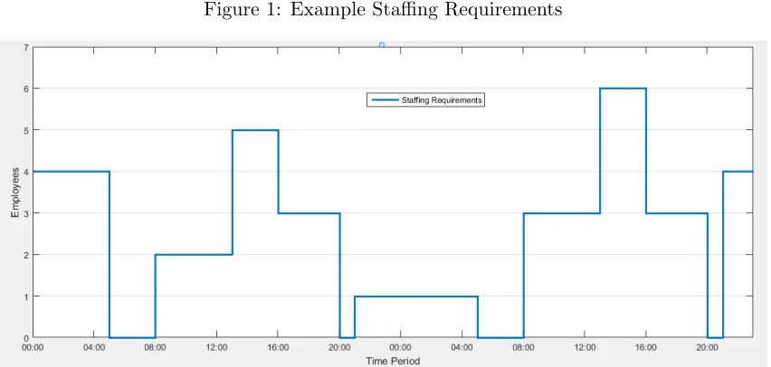
requirements, for each time period are given. Furthermore the problem is considered to be cyclic, which means that employees starting on the last day and working overnight will be considered to be active from the first time period onwards. Figure 1 shows an example of staffing requirements spread out over a two day cycle.
The requirements state how many duties are necessary in order to cope with the demand at any time period and therefore it is desired to have at least as many employees working as the requirements. On the other hand having too many employees working is a waste of resources. Therefore it is desired to follow the requirements closely. In order to mea-sure deviations from the requirements we will use the terms overstaffing and understaffing. Overstaffing counts the surplus in number of employees over the staffing requirements and understaffing counts the deficit. Both overstaffing and understaffing are allowed in the shift design problem and different importance can be put into these two factors.
Figure 1: Example Staffing Requirements
Table 1: Example Shift Types
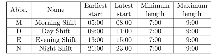
Abbr. Name Earliest
start
Latest start
Minimum length
Maximum length
M Morning Shift 05:00 08:00 7:00 9:00
D Day Shift 09:00 11:00 7:00 9:00
E Evening Shift 13:00 15:00 7:00 9:00
N Night Shift 21:00 23:00 7:00 9:00
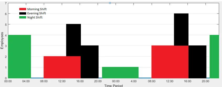
2.1 Shift Design The shifts can only be chosen based on a set ofshift types. A shift type specifies the earliest and latest starting time of a shift, as well as the shortest and longest duration of a shift. In Table 1 an example of possible shift types are shown. Using these shift types we can design three different shifts and a number of duties for each shift on each of the two days to exactly meet the requirements from Figure 1. This solution is shown in Table 2 and Figure 2.
Figure 2: Example Solution Graph
Table 2: Example Solution Table Shift
Type Start End
Duties Day 1
Duties Day 2 Morning 08:00 16:00 2 3 Evening 13:00 20:00 3 3
2.1.2 Formal Description
In this section we give a formal description of the shift design problem. First the factors describing an instance of shift design are given. Afterwards the decision variables are described. Finally we show the objective of the problem.
Instance Description
An instance of shift design can be described by the following. • D consecutive days.
• These days are spanned by nequally long consecutive time slotsT ={t1, t2, ..., tn},
The problem is cyclic hencet1 followstn.
• Staffing requirements Rt ∀t∈T.
• Set of shift types Y, each shift type,y∈Ycontains the minimum and maximum start and duration of a shift of that type:
y.min start, y.max start, y.min length, y.max length. • W1, W2 and W3 representing respectively the penalty for
overstaffing, understaffing, and the number of shifts. Decision Variables
The decision variables in the shift design problem are the following.
• A set of shiftsS, where for each s∈S we choose the type, start and length, s.type, s.startand s.length.
The start and length of each shift need to comply with the shift type hence we require s.type.min start ≤s.start ≤s.type.max start ∀s∈S s.type.min length ≤s.length ≤s.type.max length ∀s∈S • For each shift the number of duties at each day
ws,d ∀s∈S, d∈ {1, ..., D}
Objective
The objective is made up of three parts: the overstaffing, the understaffing and the num-ber of shifts. In order to calculate the overstaffing and understaffing we define the active workers for each time period represented byat ∀t∈T. atwill be equal to the number of
employees working at time periodt.
at=
X
s∈S
xs,d, wherexs,d=
(
ws,d if time slott belongs to the interval of shiftson day d
2.1 Shift Design We will useO to denote the total overstaffing andU to denote the total understaffing. We define them as follows.
O =X
t∈T
max{at−Rt,0}
U =X
t∈T
max{Rt−at,0}
The objective is to minimise the weighted sum of overstaffing, understaffing and the number of shifts.
2.2 Break Scheduling
First we will give an introduction to the break scheduling problem. The formulation that we use is taken from [33]. The break scheduling problem uses characteristics of the shift design problem and we use similar notation as in the shift design problem. Therefore we will describe break scheduling as the problem of scheduling breaks for each duty as opposed to breaks for a shift. This will allow us to smoothly combine the two separate problems to formulate the shifts and breaks design problem afterwards.
2.2.1 Introduction
The break scheduling problem considers the allocation of breaks to a workforce. In this problem the planned shifts and number of employees on each day are considered to be fixed. In the break scheduling problem we are deciding on which breaks to allocate for each duty. A break can be characterised by its starting time and the length. Various restrictions are set on the breaks. These restrictions are usually set to ensure that workers can function optimally and are based on labour rules and therefore must be satisfied.
A duty is made up of two complementary time periods namely the breaks and theworking periods. Therefore the working periods represent the time periods of a duty in which the employee is continuously working. We do however not consider a duty to beactive on the first time period following a break. Instead we consider the duty to be getting accustomed with a new working situation after their break. Hence the first time period following a break does not count towards the break time of a duty and neither to the staffing require-ments.
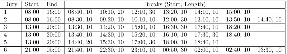
2.2 Break Scheduling Figure 3: Example Staffing Requirements
Table 3: Example Duties and Breaks Duty Start End Breaks (Start, Length)
1 08:00 16:00 08:40, 10 10:10, 20 12:10, 30 13:20, 10 14:10, 10 15:00, 10
2 08:00 16:00 08:30, 10 09:20, 10 10:10, 10 12:00, 30 13:10, 10 13:50, 10 14:40, 10 3 13:00 20:00 13:30, 10 14:20, 10 15:00, 10 16:30, 30 17:40, 10 18:20, 10
4 13:00 20:00 13:40, 10 14:30, 10 15:20, 10 16:10, 10 17:30, 30 18:40, 10 5 13:00 20:00 14:40, 20 15:30, 10 17:00, 30 18:00, 10 18:40, 10
6 21:00 05:00 21:40, 10 22:30, 10 23:10, 10 00:50, 30 02:00, 10 02:40, 10 03:30, 10
The restriction on breaks and working periods are as follows. • Total break length is fixed (depends on the length of the duty). • Breaks have a minimum and maximum length.
• Working periods have a minimum and maximum length.
• If the working periods is longer thanlong working period the next break has a higher minimum length.
• Break cannot start too early or too late for a duty so that employees is always working in the first few and last few time periods of their duty.
[image:16.612.110.571.347.435.2]2.2.2 Formal Description
In this section we give a formal description of the break scheduling problem. First we give the factors used to describe an instance of break scheduling. Afterwards the decision variables are described. Next the restrictions on feasible break patterns are specified. Finally we show the objective of the problem.
Instance Description
An instance of break scheduling can be described by the following. • A set of nequally long consecutive time slotsT ={t1, t2, ..., tn},
The problem is cyclic hencet1 followstn.
• Staffing requirements Rt ∀t.
• Set of dutiesE, Each duty ehas a starting time slot and a length, e.start, and e.length.
• W1 and W2 representing respectively the penalty for overstaffing and understaffing.
• Parameters for the constraints:
total break time( for each duty)
break minimum lengthand break maximum length
working period minimum lengthand working period maximum length long working period and long break minimum length
earliest break startand latest break start min length for lunch,lunch break length,
earliest lunch break startand latest lunch break start.
Decision Variables
For each duty we are deciding on the number of breaks, and for each break on the start and length of the break. We let e.breaksdenote the number of breaks of duty e. Furthermore we let be,i refer to theith break of duty e.
Then the decision variables are • e.breaks ∀e∈E
• be,i.start ∀i∈ {1, e.start}, e∈E
2.2 Break Scheduling be,i.startdenotes the start of the break relative to the start of dutye, i.e. be,i= 1 implies
that the ith break of dutyestarts on the 1st time period of dutye.
These variables also determine the working periods. we will usewpe,ito denote the length of
theith working period of dutye. If dutyecontainse.breaksbreaks it containse.breaks+ 1 working periods.
Restrictions
The total break time of each duty is given, we will usee.total break timeto denote this for duty e. In order to ensure exactly this amount of break time is allocated we require the following constraints.
e.breaks
X
i=1
be,i.length=e.total break time ∀e∈E (2)
A break has a minimum and a maximum length. The following constraints ensure this. break minimum length≤bi,e.length ∀i= 1, ..., e.breaks, e∈E (3)
break maximum length≥bi,e.length ∀i= 1, ..., e.breaks, e∈E (4)
Similarly, the working periods have a minimum and maximum length.
working period minimum length≤wpe,i ∀i= 1, ..., e.breaks+ 1, e∈E (5)
working period maximum length≥wpe,i ∀i= 1, ..., e.breaks+ 1, e∈E (6)
Breaks following a long working period have a different minimum length. We require this by the following implication.
wpe,i≥long working period =⇒
be,i≥long break minimum length ∀i= 1, ..., e.breaks, e∈E (7)
Breaks have an earliest and latest possible starting time.
be,i.start≥earliest break start ∀i= 1, ..., e.breaks, e∈E (8)
be,i.start≤latest break start ∀i= 1, ..., e.breaks, e∈E (9)
In case that the length of a duty is longer than the minimum length required for a lunch break, one of the breaks needs to be assigned the status of lunch break. This break has a fixed length and bounds on the earliest and latest start.
e.length≥min length for lunch =⇒ ∃i s.t. be,i.start≥earliest lunch break start ∧
be,i.start≤latest lunch break start ∧
Objective
In the break scheduling problem the objective is made up of two parts: the overstaffing and the understaffing. In this section we define the active workers again which has a different meaning as compared to the shift design problem. However the implication of the active workers remains: it is the number of employee who are present and actively working at each time period.
at=
X
e∈E
xt,e, wherext,e=
1 if time slot tbelongs to the interval of duty eand the duty is not on break on period t or period t-1 0 otherwise
A duty is not active on the time period after a break since we assumed that this time period is used to acclimatize to new working conditions after returning from a break. As in the shift design problem we will use O to denote the total overstaffing and U to denote the total understaffing. We define them as follows.
O=X
t∈T
max{at−Rt,0}
U =X
t∈T
max{Rt−at,0}
The objective is to minimise the weighted sum of overstaffing and understaffing.
2.3 Shifts and Breaks Design 2.3 Shifts and Breaks Design
In this section we start with an introduction to the shifts and breaks design problem. Afterwards we will give a formal description of the problem. We follow the formulation used by [15].
2.3.1 Introduction
The shifts and breaks design problem combines the shift design and the break scheduling problem. The staffing requirements over a planning horizon are given. The goal of the problem is to find a small set of shifts with a number of duties allocated to each shift on each day, and a break allocation to each duty, such that the staffing requirements are closely followed.
The shifts can be chosen from a set of shift types as outlined in the shift design prob-lem. There are many restrictions set on a feasible break allocation as is described in the break scheduling problem.
2.3.2 Formal Description
First we will list the factors which describe an instance of shifts and breaks design. After-wards we define the decision variables of the problem. In the next section we will state the restrictions on the decision variables. Finally we give the objective function.
Instance Description
• D Consecutive days.
• These days are spanned by nequally long consecutive time slotsT ={t1, t2, ..., tn},
The problem is cyclic hencet1 follows tn.
• Staffing requirements Rt ∀t.
• Shift types y ∈Y, each shift type contains the minimum and maximum length and duration of a shift of that type:
y.min start, y.max start, y.min length, y.max length. • W1, W2 and W3 representing respectively the penalty for
overstaffing, understaffing, and the number of shifts.
• parameters for the constraints on breaks:
break minimum lengthand break maximum length
working period minimum lengthand working period maximum length long working period and long break minimum length
earliest break startand latest break start min length for lunch,lunch break length,
earliest lunch break startand latest lunch break start.
Decision Variables
In this problem we are designing the shifts. For each shift we decide on the number of duties it will have on each day. Furthermore for each of these duties we decide on their break allocation. We use the following decision variables regarding the design of the shifts. • A set of shiftsS, where for each shift s∈S we decide on the type, start and length,
s.type, s.start ands.length.
• For each shift the number of duties at each day, ws,d ∀s∈S, d∈ {1, ..., D}.
We will usesd,e.breaksto denote the number of breaks for dutyestarting on daydof shift
s. Furthermore we let bs,d,e,i refer to the ith break of duty estarting on day dof shift s.
Then the decision variables regarding the breaks are the following. • sd,e.breaks ∀s∈S, d∈ {1, ..., D}, e∈ {1, ..., ws,d}
• bs,d,e,i.start ∀s∈S, d∈ {1, ..., D}, e∈ {1, ..., ws,d}, i∈ {1, ..., sd,e.breaks}
• bs,d,e,i.length ∀s∈S, d∈ {1, ..., D}, e∈ {1, ..., ws,d}, i∈ {1, ..., sd,e.breaks}
Restrictions
The shifts need to be of a type as defined in the input and the start and length of each shift need to comply with its type. Hence we require the following constraints.
s.type.min start≤s.start≤s.type.max start ∀s∈S s.type.min length≤s.length≤s.type.max length ∀s∈S
Furthermore a set of restrictions is placed on the break allocation of each duty. The total break time of each shift is given byf(s) and the break time allocated to each duty of this shift needs to be equal to this.
es,d.breaks X
i=1
2.3 Shifts and Breaks Design The following constraints need to hold for all breaks, which means the constraints should hold ∀s∈S, d∈ {1, ..., D}, e∈ {1, ..., ws,d}, i∈ {1, ..., es,d.breaks}
bs,d,e,i.length≥break minimum length (13)
bs,d,e,i.length≤break maximum length (14)
wps,d,e,i≥working period minimum length (15)
wps,d,e,i≤working period maximum length (16)
wps,d,e,i≥long working period =⇒
bs,d,e,i≥long break minimum length (17)
bs,de,i.start≥earliest break start (18)
bs,d,e,i.start≤latest break start (19)
(20) Lastly, for each shift of sufficient length, all duties need to be allocated a lunch break.
e.length≥min length for lunch =⇒ ∃is.t.
bs,d,e,i.start≥earliest lunch break start ∧
bs,d,e,i.start≤latest lunch break start ∧
bs,d,e,i.length=lunch break length ∀s∈S, d∈ {1, ..., D}, e∈ {1, ..., ws,d}
(21) Objective
The objective function is the weighted sum of overstaffing understaffing and the number of shifts. In order to define the overstaffing and understaffing we define theactive workers
again. We use the notation e∈sd to denote the duties which are part of shift sand start
on day d. at=
X
s∈S
xs,d, where
xs,d=
(
ws,d−Pe∈sdye,t, iftbelongs to the interval of the duties of shift sthat start on dayd
0 otherwise
ye,t=
(
1 if duty eis on a break in tor t−1 0 otherwise
Using the active workers we define the overstaffing and understaffing which lead to the objective function. We will use O to denote the total overstaffing and U to denote the total understaffing. We define them as follows.
O=X
t∈T
max{at−Rt,0}
U =X
t∈T
max{Rt−at,0}
The objective is to minimise the weighted sum of overstaffing, understaffing and the number of shifts.
3
Literature Review
This section is split up into four different parts. In the first part we will give an overview of literature regarding personnel scheduling. We will also note the differences between most available literature regarding personnel scheduling problems and the shifts and breaks design problem. Afterwards we will give an overview of literature directly related to the shift design problem as discussed in this thesis. Next we will do the same for the break scheduling problem and finally we will give an overview of literature directly related to the shifts and breaks design problem.
3.1 Personnel Scheduling
of the model and tested instances for which exactly three breaks were required for each duty, having a combined duration of two hours. Furthermore, the second break was re-quired to be the longest break and the continuous periods in-between two breaks (working period) was restricted to have a length between one and three hours. For this problem Rekik et al. [30] propose two integer linear program formulations and compare their results with modified versions of integer linear programming formulations given by Bechtold and Jacobs [5] and Aykin [2]. Rekik et al. [30] show that their model is slightly slower than the formulations in [5] and Aykin [2] which is explained by the added flexibility that their model gives. The slight modification considered of the model proposed by Bechtold and Jacobs [5], show that this modified model gives better results than the model proposed by Aykin [2] which is opposed of findings by Aykin [3] who compared the unmodified models. A recent overview of personnel scheduling is given by Van den Bergh et al. [31]. The authors note that a wide range of solution methods are used to find solution to person-nel scheduling problems. The two main approaches used are mathematical programming methods such as linear programming, goal programming, integer programming and column generation, and heuristic methods such as simulated annealing, tabu search and genetic algorithms. Other approaches include simulation, constraint programming and queueing. The shifts and breaks design problem is different from problems discussed in the liter-ature. In this problem shifts have to be designed, instead of duties, in such a way that the shifts can be efficiently reused over multiple days instead of just a single day. Furthermore the formulation allows for a large number of breaks in the shifts (up to 10 breaks for the real-life instances). An overview of literature regarding shift design and break scheduling is given by Di Gaspero et al. [16].
3.2 Shift Design
The shift design problem was first introduced by [28]. The authors make use of local search to find a solution. Tabu search [19] is used to guide the local search. The authors state that they rely on local search techniques because the shift design problem is proven to be NP hard [23], as well that there exists a constantc <1 such that approximating the shifts design problem withinclnnis NP hard (here nrefers to the total number of time periods in shift design). The authors also use domain knowledge during the search by identifying shifts during the longest period of shortage/excess and trying to improve these shifts. Fur-thermore a ’good’ initial solution is constructed. The main idea for this good solution is that time points in which the demand drastically rises (falls) needs to be a time point for shift starts (ends).
3.3 Break Scheduling heuristic is based on the relation of the shift design problem to a flow problem as described in [23]. A polynomial min cost max flow problem can be used to compute optimal staffing with weighted cost on the overstaffing and understaffing. This approach does however not minimize the number of shifts used. Furthermore this approach can only be used when cyclicity is not considered in the problem. The authors still consider a cyclic problem and do so by making different calls to the greedy heuristic where in each call only a subset of the shifts is considered so that the problem is not cyclic. For the local search algorithm the authors consider less neighbourhood relations as compared to [28]. It should be noted that the problem described in this paper is slightly different to the one described in [28]. Namely in the (chronologically) first article the objective function covers an additional term: a penalty for the distance of the average number of duties per week. This term is meant to penalise a set of shifts in which the workload is divided into many small shifts. In the later article the authors note this difference and state that, ”In practice further op-timization criteria clutter the problem. [...] Fortunately, this and most further criteria can easily be handled by straightforward extensions of the heuristics described in this paper.” Bonutti et al. [7] formulate a variation on the shift design problem. Their formulation extends the shift design problem to have multiple types of skills for employees. The re-quirements at each time period state the required number of employees at each time period for each skill. For each shift the number of workers for each day and each skill have to be specified. Furthermore in this formulation it is possible for shifts to contain a single break. Local search is used for this problem and the neighbourhood relations are an extension on the relations used in Di Gaspero et al. [14]. Furthermore simulated annealing [22] is used to guide the search process.
Answer Set Programming (ASP) [8] is an exact solution technique and has been applied to shift design by Brewka et al. [8]. ASP is able to find most best known solutions within 60 minutes on instances of shift design where those solutions have no overstaffing and under-staffing. While the execution times are often not competitive with results from [14] there are instances on which ASP works very well. Solutions found for the instances in which a solution without overstaffing and understaffing might not exist are not competitive with results from the literature. The authors state that a combination of ASP together with domain-specific heuristics is a promising area for further research.
3.3 Break Scheduling
guided by either tabu search, simulated-annealing, or a minimum conflicts-based heuristic [24]. The best results are obtained by using a minimum conflicts-based heuristic. Beer et al. [6] conclude that the two different initial solutions did not have a significant impact on the solution quality.
A memetic algorithm for break scheduling was proposed by Musliu et al. [29]. Memetic algorithms combine population based method with local search techniques and were first mentioned in [25]. The memetic algorithm keeps a number of individuals, the population, each representing a solution to the break scheduling problem. An individual is made up of memes, in this formulation each meme representing a duty. At each iteration of the algorithm the best individual is kept unaltered for the next iteration. A subset of the other individuals are chosen and either a crossover or mutation operator is applied to each individual in this subset. The crossover operator takes as input two individuals (the second being random) and outputs an individual (offspring) which inherits a part of the solution (memes) of each input (parent). The mutation operator performs a random move on an individual chosen using a local search approach. After this local search is used to improve themfittest individuals at each iteration. The authors compare their results with the min-imum conflicts-based heuristic as proposed by Beer et al. [6]. The algorithms both score best on half of the test instances and hence conclusions regarding the better algorithm are indecisive.
3.4 Shifts and Breaks Design 3.4 Shifts and Breaks Design
The shifts and breaks design problem is introduced in [15]. The authors state that to the best of their knowledge the whole problem as described in their paper has not been addressed in the literature. Various similar problems have been discussed in the literate as described in section 3.1. The authors propose an approach combining local search (LS) and constraint programming (CP) [1]. Their approach starts of with finding an initial randomly generated solution for the assignment of shifts. LS is employed on a part of the solution, namely a solution which specifies the shifts, the number of duties for each shift on each day, and the number of breaks for each duty. The CP model uses this information to try to find a break allocation within a time limit. For each iteration of the algorithm a random move is chosen which changes either the start or end of a shift by one time unit, the number of duties of a single day for a shift by one duty, the number of breaks for all duties on a single day of a shift, or by merging two shifts together. This new solution is given to the CP model and after the break allocation is determined this new solution is accepted if the objective value is better than the objective value before the random move. The algorithm fixes a part of the break variables in the CP model when a solution to the full program cannot be found in a timely manner.
4
Shift Design
In this section we will first give an integer linear program (ILP) formulation for the shift design problem. Afterwards we will describe the set of problem instances used to test the effectiveness of this ILP formulation for the shift design problem. Finally we will use the commercially available optimisation package Cplex [10] to solve instances available in the literature and compare our results to results obtained by Di Gaspero et al. [14]. A modi-fied version of the ILP for shift design will also be used in the first phase of our solution approach to the Shifts and Breaks Design problem.
4.1 ILP Shift Design
In this section we give an integer linear programming formulation to the shifts design prob-lem. A compact overview of this ILP is given in the appendix (9.1). We use this ILP to find results to the shift design problem in Section 4.3. A modified version of this ILP is also used in the first phase of our algorithm to the shifts and breaks design problem. The shift design problem is made up of time periods, days and shifts. We will use the following variables to refer to a single element of each set.
• t refers to a single time period.
• drefers to a single day.
• srefers to a single shift.
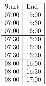
Table 4: Possible Shifts Start End 07:00 15:00 07:00 15:30 07:00 16:00 07:30 15:30 07:30 16:00 07:30 16:30 08:00 16:00 08:00 16:30 08:00 17:00
For each shift we are making the decision of using it or not. In the case that a shift is used, we call it active and we can assign a number of duties to it on each day. For these decisions we introduce the following variables.
as=
(
1 if shift sis active 0 otherwise
wd,s= the number of duties of shiftsstarting on day d
If a shift is inactive the number of duties on each day are forced to be 0. To model this constraint we use the parameter M = maxt{Rt}. Recall that Rt denotes the staffing
requirements at time periodt. Note that using more duties than this number will lead to unnecessary overstaffing. The following constraints force the number of duties to be 0 in case the corresponding shift is not active.
wd,s≤M·as ∀d, s (23)
Using the number of duties for each shift we can can calculate the overstaffing and the understaffing. For this we need a parameter denoting on which time periods the duties of a shift starting on a specific day are active. We introduce the following.
ot= the amount of overstaffing at time periodt, ot≥0
ut= the amount of understaffing at time period t, ut≥0
As,d,t=
(
1 if the duties of shift sstarting on day dare active on time periodt 0 otherwise
The following constraints specify, respectively, the understaffing and the overstaffing.
X
s,d
As,d,t·wd,s
4.2 Problem Instances ot=
X
s,d
As,d,t·wd,s
+ut−Rt ∀t (25)
In an optimal solution ifut>0 then (24) will be an equality. To see this note that if the
left hand side would be strict then we could decrease ut which would decrease the
objec-tive. The objective function is the weighted sum of the overstaffing, understaffing and the number of shifts.
Results of this ILP on instances of shift design are given in Section 4.3. In our two-phase approach to the Shifts and Breaks design problem we use a modified version of this ILP. The modified ILP is based on using virtual shifts which will be described in the next section.
minimizeW1X
t
ut+W2
X
t
ot+W3
X
s
as (26)
4.2 Problem Instances
Table 5: Shift Types
Abbr. Name Earliest
start
Latest start
Minimum length
Maximum length
M Morning Shift 05:00 08:00 7:00 9:00
D Day Shift 09:00 11:00 7:00 9:00
E Evening Shift 13:00 15:00 7:00 9:00
N Night Shift 21:00 23:00 7:00 9:00
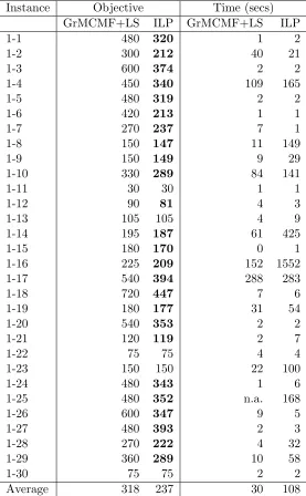
4.3 Results
The integer linear program for shift design was written in C++ using Microsoft Visual Studio 2013 [9], using the commercially available optimisation package Cplex [10] to solve it.
In this section we compare the results of our ILP approach to the results obtained by Di Gaspero et al. [14]. Overall the authors found their best results using a combination of a greedy min-cost max-flow formulation and local search. The authors refer to this approach by ’GrMCMF+LS’. We compare our results to the results of GrMCMF+LS. For the instances of the first data set the authors were interested in the time it took for their approach to reach the ’best known’ solutions of shift design. The best known solutions are equal to either the solution used for constructing the instance or a better so-lution as found in their article. The authors report average running time of their algorithm to obtain the best known solutions. For one of the instances GrMCMF+LS was unable to find the best known solution.
4.3 Results the found solution and gap of this solution. In Cplex the gap is defined as
|bestnode−bestinteger|
10−10+|bestinteger| (27)
where bestnode is a lowerbound to the problem, a solution of a linear relaxation of the ILP, and bestinteger is the current best solution to the ILP. Thus the gap is the ratio of a difference between the best found solution and a lowerbound divided by the lowerbound. For the ILP with a time limit of 30 minutes we also report the found solution and the gap, indicated by ’ILP+’. We also report the running time of the ILP in seconds, which can be lower than 1800 if the optimal solution is found.
Table 6: Shift Design Comparison Set 1
Instance Objective Time (secs)
GrMCMF+LS ILP GrMCMF+LS ILP
1-1 480 320 1 2
1-2 300 212 40 21
1-3 600 374 2 2
1-4 450 340 109 165
1-5 480 319 2 2
1-6 420 213 1 1
1-7 270 237 7 1
1-8 150 147 11 149
1-9 150 149 9 29
1-10 330 289 84 141
1-11 30 30 1 1
1-12 90 81 4 3
1-13 105 105 4 9
1-14 195 187 61 425
1-15 180 170 0 1
1-16 225 209 152 1552
1-17 540 394 288 283
1-18 720 447 7 6
1-19 180 177 31 54
1-20 540 353 2 2
1-21 120 119 2 7
1-22 75 75 4 4
1-23 150 150 22 100
1-24 480 343 1 6
1-25 480 352 n.a. 168
1-26 600 347 9 5
1-27 480 393 2 3
1-28 270 222 4 32
1-29 360 289 10 58
1-30 75 75 2 2
4.3 Results
Table 7: Shift Design Comparison Set 3
Instance Objective Gap Time (secs)
GrMCMF+LS ILP ILP+ ILP ILP+ ILP+
3-1 2386 318 318 0.31 0 8
3-2 7691 845 536 0.58 0 87
3-3 9597 924 542 0.55 0 25
3-4 6681 1427 500 0.77 0 119
3-5 9996 551 508 0.28 0 5
3-6 2077 1892 315 0.89 0 65
3-7 6087 642 585 0.28 0 72
3-8 8861 725 537 0.45 0 47
3-9 6036 2527 570 0.83 0 420
3-10 3002 462 366 0.52 0 62
3-11 5491 1024 474 0.73 0 195
3-12 4171 3514 520 0.91 0.04 1800
3-13 4662 3131 535 0.89 0.07 1800
3-14 9661 701 461 0.42 0 3
3-15 11445 1112 641 0.57 0 151
3-16 10734 638 477 0.38 0 3
3-17 4729 3011 523 0.89 0.04 1800
3-18 6692 893 526 0.67 0 200
3-19 5157 2677 594 1 0.13 1800
3-20 9175 1845 606 0.80 0 232
3-21 6054 4674 718 1 0.10 1800
3-22 12870 2063 720 0.76 0.03 1800
3-23 8390 699 630 0.42 0 18
3-24 10418 741 590 0.43 0 5
3-25 13252 847 635 0.41 0 5
3-26 13118 1042 724 0.50 0 193
3-27 10081 1034 633 0.56 0 7
3-28 10604 887 539 0.53 0 5
3-29 6690 1045 571 0.69 0 263
3-30 13724 1011 607 0.53 0 6
5
Break Scheduling
In this section will formulate a solution approach to the break scheduling problem. We will first formulate the problem of assigning an optimal break allocation for a single duty as an integer linear program. Afterwards we state how this problem can be modified so that multiple duties can be considered at the same time. We will propose two algorithms which use these ILP models to find break patterns for all duties. We will compare results of both our algorithms as well as results obtained by Widl and Musliu [33].
5.1 ILP Break Scheduling Single Duty
In this section will formulate the problem of optimally allocating the break allocation for a single duty. A compact overview of this ILP is given in the appendix 9.2.
First we will define the set of possible breaks for a duty. Since the total break time for a duty is given, as well as the minimum break length, we can calculate the maximum possible number of breaks in a duty. We letMbreaksbe this maximum number of breaks+1.
The 1 is added such that we can use the same set to denote the working periods, since there is always 1 more working period than breaks. We use the following set to enumerate all breaks.
B ={1,2, ..., Mbreaks} (28)
For each (possible) break we first need to decide whether the break will be active, and in case a break is active we need to decide the starting period and the length of the break. We use the binary variables ab to indicate whether break bis active. First we impose the
following constraint which force the breaks to be in chronological order since a break can only be active if the previous break was also active.
ab ≤ab−1 ∀b∈B\ {1} (29)
Breaks following a long working period are considered different since they have a different minimum length. Furthermore, one of the breaks (might) need to be assigned the status of lunch break, which requires it to be somewhere in the middle of the duty and have a specific length. We will use the binary variables alb to indicate whether break b needs to be long, and the binary variables lb to denote whether break b is assigned the status of
lunch break. Only active breaks can be long or lunch and therefore we require the following constraint.
alb+lb ≤ab ∀b∈B (30)
We use integer variables blb to denote the length of the bth break in number of time peri-ods. Since the total break time (T bt=total break time) is given we require the following constraint.
X
b
blb =T bt (31)
In order to enforce some of the logical constraints we will use M to denote a sufficiently large variable, in this caseM will be equal to the length of the duty expressed in number of time periods. First we set a minimum and maximum length on the breaks, usingBminl= break minimum length and Bmaxl = break maximum length, on all active break lengths. Note that the length of inactive breaks gets forced to 0. The lunch break length might exceed the maximum normal break length hence we also account for this by making the constraint inactive for the break assigned the status of lunch break.
M·(1−ab) +blb ≥Bminl ∀b∈B (32)
blb ≤Bmaxl·ab+M·lb ∀b∈B (33)
Long breaks will have a different minimum length. This is specified by the following constraint using Lbml=long break minimum length.
alb·Lbml≤blb ∀b∈B (34)
The variables bsb will correspond to the start of break b i.e. the first time period on which the respective break is active. We use t to refer to the time periods in this ILP. Later we will introduce constraints such that the break start is forced to be on a time period. Using that the duty lasts a total of Length time periods, the set of time periods is given by
T ={1,2, ..., Length} (35)
Breaks can not start too close to the shift extremes (Ebs = earliest break start and Lbs = latest break start). Therefore we add the following constraints which are only active for active breaks.
bsb ≥Ebs ∀b∈B (36)
bsb ≤Length−Lbs+ (1−ab)·(Lbs+ 1) ∀b∈B (37)
Constraint (37) combined with Constraint 38 ensures that the break start of inactive breaks is set to the first time period following the shift end. This is useful for defining the working periods.
bsb ≥(Length+ 1)·(1−ab) ∀b∈B (38)
We let the variables wpb denote the length (in time periods) of the bth working period.
5.1 ILP Break Scheduling Single Duty before the first break starts. For the other working periods, the bth working period start after the b−1th break has ended and ends when break bstarts.
wp1 =bs1−1 (39)
wpb =bsb −(bsb−1+blb−1) ∀b∈B\ {1} (40) Active working periods have a lower and upper bound on their length. These are given by the parameters W pminl=working period minimum lengthand
W pmaxl = working period maximum length. Note that a working period wpb is
active if break b−1 is active, and thatwp1 is always active.
wpb ≤W pmaxl ∀b∈B (41)
wp1 ≥W pminl (42)
M ·(1−ab−1) +wpb ≥W pminl ∀b∈B\ {1} (43)
The following constraints ensure, respectively, that alb or lbis forced to 1 if break b
fol-lows a long working period and to 0 otherwise. Hereto we use the parameter M lwp = minimum long working period. We have earlier specified that a break can be either long or lunch, and only if it is active, and therefore we let the first constraint be inac-tive for the break which is the lunch break. By doing this we make the assumption that minimum long working period ≤ lunch break length. The constraint is also inac-tive for inacinac-tive breaks, this is necessary because otherwise we could force an inacinac-tive break to be long which is not feasible.
wpb−M lwp+ 1≤alb·M +lb·M+ (1−ab)·M ∀b∈B (44)
M lwp−wpb≤(1−alb)·M ∀b∈B (45)
If a lunch break is required there needs to be exactly one lunch break. We will use the parameter L which will be equal to 1 if a shift needs a lunch break and 0 otherwise. We have already introduced lb, indicating whether a break is the lunch break. Therefore we
require the following.
X
b
lb =L (46)
A lunch break has a fixed length of Lbl = Lunch break length, a minimum start at
Elbs=Earliest lunch break start, and a maximum start atLlbs=Latest lunch break start. In order to ensure that the break which will be the lunch break does not violate any of these
constraints we add the following four types of constraints. Respectively the constraints en-sure that the lunch break does not: last shorter than allowed, last longer than allowed, start earlier than allowed, and that the lunch break does not start later than allowed.
(1−lb)·M ≥blb−Lbl ∀b∈B (48)
(1−lb)·M ≥Elbs−bsb ∀b∈B (49)
(1−lb)·M ≥bsb −Llbs ∀b∈B (50)
Up until this point we have defined variables which specify all breaks. What is left is to define variables for the overstaffing and understaffing. To do this we need to specify whether the duty is active at a time period. In order to do this we add binary variables zst∗,b and zte∗,b. Note that we uset∗ to index these variables rather thant. This is done to
highlight the fact that, since inactive breaks have their break start and break end one time period after the last time period of the duty, an additional time period is needed for these variables. Therefore we use the set T∗ for these variables instead of T where
T∗={1,2, ..., Length, Length+ 1} (51)
zts∗,b=
(
1 if time period t∗ is the first time period on which thebth break is active 0 otherwise
zte∗,b=
(
1 if time period t∗ is is the last time period on which thebth break is active 0 otherwise
All other variables of the ILP can be derived from these two types of variables since they specify all breaks. Furthermore the variables zst∗,b, zte∗,b, ab, alb, and lb are the only binary
variables in the ILP model. The other variables, such as the break start bs
b and the break
length blb can be relaxed to be continuous. We will add constraints to ensure that these variables only take on integer values.
We use the following 4 types of constraints to determine the break start and length using the variables zts∗,b and zte∗,b. Constraint (52) ensures that exactly 1 time period is taken
as the break start. Constraint (53) constraint ensures that the continuous variables bs b are
correctly taken based onzts∗,b. Constraint (54) ensures that exactly 1 time period is taken
as the break end. Constraint (55) ensures that the continuous variables blb are correctly taken based on zet∗,b, note that the term 1−ab is needed to correct the constraint for
inactive breaks since inactive breaks have a length of 0.
X
t∗
zst∗,b= 1 ∀b∈B (52)
X
t∗
5.1 ILP Break Scheduling Single Duty
X
t∗
zet∗,b= 1 ∀b∈B (54)
X
t∗
t∗·zet∗,b=bsb +blb−1 + (1−ab) ∀b∈B (55)
The following two types of continuous variables are used to determine whether a duty is on a break in a time period. This is necessary for verifying whether a duty is active on a time period. We use the following variables.
zt,bb =
(
1 if time period tis before the start of the bth break 0 otherwise
zt,ba =
(
1 if time period tis after the bth break has ended 0 otherwise
The following two constraints ensure that these variables take on the correct value. Con-straint (56) ensures that zt,bb is correctly defined, note that a time period is before a break if the break start is after the time period. Constraint (57) ensures that zat,b is correctly defined, note that a time period is after a break if the break end is before the time period.
Length+1 X
i=t+1
zi,bs =zt,bb ∀t∈T, b∈B (56)
t−1 X
i=1
zi,be =zt,ba ∀t∈T, b∈B (57)
We will use the variableszt,b denote whether the duty is on itsbth break on time periodt.
A duty is on its bth break at time periodtif the time period is not before the break start and not after the break end. We have already introduced variables to indicate these cases and since a time period is either before a break, during a break, or after a break we use the following constraint to determine zt,b.
zt,b+zt,ba +zt,bb = 1 ∀t∈T, b∈B (58)
xtwill indicate whether the duty is active on time period t. This is true if and only if the
periods of the duty to be active in case the duty is not on any break and no break ended the previous time period.
1−xt≥
X
b
zt,b ∀t∈T (59)
1−xt≥
X
b
zte−1,b ∀t∈T \ {1} (60)
1−x1≤X
b
z1,b (61)
1−xt≤
X
b
zt,b+
X
b
zet−1,b ∀t∈T (62)
The last variables we define are the overstaffing and understaffing variables. These will be used in the objective function. For this ILP we assume that the allocation of other shifts is fixed. This fixed allocation together with the assumption that the duty, for which the breaks are to be decided, takes no breaks, make up the fixed staffing. Let us use Dt
to determine the demand at time period t which is a parameter used in this ILP. Dt is
equal to the requirements at period t minus the fixed staffing at period t. Note that the duty considered in the ILP is considered to have no breaks while determining the fixed staffing. We use the following two (in)equalities to base the overstaffing and understaffing constraints on.
fixed staffing +xt−1 + understaffing≥requirements
overstaffing =xt−1 + understaffing + fixed staffing−requirements
Then the following constraints specify the over and understaffing, using ot to define the
overstaffing at time periodt and ut to define the understaffing at time periodt.
xt−1 +ut≥Dt ∀t∈T (63)
ot−ut−xt+ 1 =−Dt ∀t∈T (64)
ot, ut≥0 (65)
Finally we specify the objective function. minimizeW1X
t
ot+W2
X
t
ut (66)
5.2 ILP Break Scheduling Multiple Duties
5.3 Algorithms for Break Scheduling day of a shift. For this ILP all variables as described in the previous section, except for the understaffing and overstaffing, need an additional subscript eindicating the duty. Then all constraints except the constraints specifying understaffing, Constraint 63, and overstaffing, Constraint 64, need to hold for all duties. These two mentioned constraints should be replaced by the following constraints.
X
e
xt,e−1
+ut≥Dt ∀t∈T (67)
ot,e−ut,e−
X
e
xt,e+ 1
=−Dt ∀t∈T (68)
5.3 Algorithms for Break Scheduling
In this section we will propose two algorithms used to allocate all breaks using the break scheduling ILP’s from the previous two sections. The first algorithm will only use the break ILP model from Section 5.1 which allocates the break pattern for a single duty. The second algorithm will also use the ILP from section 5.2 and use it to find the optimal break allocation for two duties at the same time. In Section??we compare results of these two algorithms on instances of break scheduling. After introducing the two algorithms we will show a way to improve the running time of both algorithms by not considering the break allocation of duties for which nothing changed since their break allocation was last considered.
5.3.1 Using Single Duties
We will give a short description of the algorithm used to allocate all break allocations using only the ILP model from Section 5.1. Pseudocode of this algorithm is also shown. The algorithm starts with a random duty and assigns a break allocation as specified by the solution of the break scheduling ILP for a single duty. Afterwards the number of active workers at each time period is updated and a break allocation is found for the next duty. After all duties have been considered by this approach the algorithm starts over again with the first duty. This process continuous until all duties have been considered in a row without the objective function of the break scheduling problem changing.
Algorithm 1 shows the pseudocode for this algorithm. We use E to denote the set of all duties. SinceE contains all duties we can use it to determine the initial Active Workers (assuming no breaks). We will use Obj(E) to denote the objective value to the shifts and breaks design problem using the duties in E (and their possible break allocation).
5.3.2 Using Double Duties
InitialiseActive W orkers usingE (assuming no breaks) Current Objective=Obj(E)
P revious Objective=∞
whileCurrent Objective<Previous Objective do fore∈E do
if e has a break allocation then remove break allocation from e updateActive W orkers end
Solve Break Scheduling ILP for dutyeusing Active W orkers Use solution from ILP to allocate breaks to e
updateActive W orkers end
Previous Objective=Current Objective Current Objective=Obj(E)
end
Algorithm 1:Second Phase Algorithm Using Single Duties
duty has a break allocation we will use the ILP from Section 5.2 to optimally allocate the breaks for two duties at the same time. Hereto we first search for any pair of two duties, having same start time and length, and having at least one time period in common in which there is understaffing and both of the duties are inactive. Since the duties need to have the same starting time and length the duties have to belong to the same shift and day. The reasoning for looking for duties satisfying these properties is that time periods with understaffing are where most of the improvements can be found since the penalty for understaffing is higher in our instances than the penalty for overstaffing. We keep doing this until there is no such pair of duties, or until all shifts and days have been considered in a row without finding improvements.
Pseudocode for this algorithm is shown in Algorithm 2. We will use S to denote the set of all shifts andDto denote the set of all days. In the pseudocode we use the following notation.
T(s, d) Time periods belonging to the duties of shift sstarting on dayd E(s, d) Duties of shiftsstarting on day d
e(t) =
(
5.3 Algorithms for Break Scheduling
Initialise Active W orkersusingE (assuming no breaks) fore∈E do
Solve Break Scheduling ILP for dutyeusing Active W orkers Use solution from ILP to allocate breaks to e
updateActive W orkers end
Current Objective=Obj(E) P revious Objective=∞
whileCurrent Objective<Previous Objective do for s∈S do
ford∈Ddo fore∈Es,d do
for e0 ∈Es,d\ {e} do
if t∈Ts,d where e(t) +e0(t) = 0 then
remove break allocation fromeand e0
Solve Break Scheduling ILP Multiple duties foreand e0 Use solution from IP to allocate breaks ofeand e0 update Active Workers
end end end end end
Previous Objective=Current Objective Current Objective=Obj(E)
end
5.3.3 Improvement
Both algorithms naively loop over all duties. However each duty only influences a subset of the time periods on the planning horizon. During the first round of the while loop all duties should be considered as they all obtain a new break allocation. However it might be possible that there is a single duty which has no time periods overlapping with another duty. It would be useless to consider this duty again in the next while loop since the fixed staffing has not changed and hence the break scheduling ILP will return the same solution. It is also possible that during the third round of the while loop some duties are considered for the break ILP but the fixed staffing of the time periods of that duty have not changed to the situation in the second while loop. In this case we also do not have to solve the break allocation ILP since we already know the optimal solution.
In order to check whether the fixed staffing for the break scheduling ILP of a duty has changed we will keep track of the variablesFt,e which we define as follows.
Ft,e=
(
1 if time period t is part of dutye and the break allocation has changed last iteration 0 otherwise
We use these variables to check whether we will solve a break scheduling problem for a duty or not. We will solve a break scheduling problem for dutyeif there exists at least one other duty which has at least one time period in common with duty e and for which the break allocation changed in the last iteration. By abuse of notation we will write t∈eto denote that time periodtis part of dutye. Using these variables we can rewrite Algorithm 1 to Algorithm 3 which is shown on the next page.
5.4 Problem Instances
5.4 Problem Instances
Initialise Active W orkersusingE (assuming no breaks) Current Objective=Obj(E).
P revious Objective=∞; Ft,e= 1 ∀t, e
whileCurrent Objective<Previous Objective do fore∈E do
if ∃ e06=es.t. Ft,e0 = 1 and t∈ethen
if e has a break allocation then remove break allocation from e updateActive W orkers end
Solve Break Scheduling ILP for duty eusingActive W orkers Use solution from ILP to allocate breaks to e
UpdateActive W orkers UpdateFt,e ∀t.
end end
P revious Objective=Current Objective Current Objective=Obj(E).
end
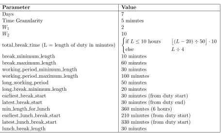
Table 8: Parameters
Parameter Value
Days 7
Time Granularity 5 minutes
W1 2
W2 10
total break time (L = length of duty in minutes)
(
ifL≤10 hours
(L−20)÷50 ·10
else L÷4
break minimum length 10 minutes
break maximum length 60 minutes
working period minimum length 30 minutes working period maximum length 100 minutes
long working period 50 minutes
long break minimum length 20 minutes
earliest break start 30 minutes (from duty start)
latest break start 30 minutes (from duty end)
min length for lunch 360 minutes (6 hours)
earliest lunch break start 210 minutes (from duty start) latest lunch break start 330 minutes (from duty start)
lunch break length 30 minutes
The parameters defining these instances are given in 8. For the break scheduling ILP, these parameters allow for a total of 336,599 possible break allocations for duties with a length of 7 hours and duties with a length of 8 hours have 1,878,678 possible break allocations. These numbers were found by initialising a break scheduling ILP to Cplex with an empty objective value. Cplex offers a populate method which can be used to find all optimal solutions. Since the objective function is empty all feasible solutions are optimal. We also tried this method to find the number of feasible break allocations for duties of length 9. After 30 minutes Cplex found over 6,000,000 possible solutions, however at this point we interrupted the search so more solutions might be possible.
A solution to the break scheduling problem corresponds to exactly one break allocation. This can be verified by noting that the variables ab, lb, blb, and bsb uniquely define a
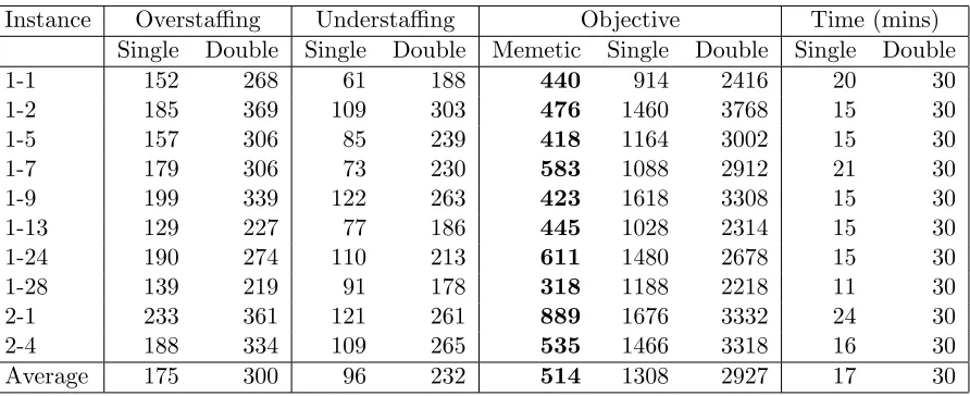
5.5 Results Table 9: Results Break Scheduling
Instance Overstaffing Understaffing Objective Time (mins)
Single Double Single Double Memetic Single Double Single Double
1-1 152 268 61 188 440 914 2416 20 30
1-2 185 369 109 303 476 1460 3768 15 30
1-5 157 306 85 239 418 1164 3002 15 30
1-7 179 306 73 230 583 1088 2912 21 30
1-9 199 339 122 263 423 1618 3308 15 30
1-13 129 227 77 186 445 1028 2314 15 30
1-24 190 274 110 213 611 1480 2678 15 30
1-28 139 219 91 178 318 1188 2218 11 30
2-1 233 361 121 261 889 1676 3332 24 30
2-4 188 334 109 265 535 1466 3318 16 30
Average 175 300 96 232 514 1308 2927 17 30
5.5 Results
The algorithm for breaks scheduling was written in C++ using Microsoft Visual Studio 2013 [9]. The integer linear programs were solved using the commercially available optimi-sation package Cplex [10].
For break scheduling we compare algorithms 1 and 2 which we refer to by ’Single’, and ’Double’, respectively. Recall that the ’Single’ algorithm only considers the break allocation for a single duty at a time and the ’Double’ algorithm also considers the break allocation for two duties. For both algorithms we also used to variables Ft,e to skip unnecessary
break scheduling ILP’s. In Table 9 results are shown. We also show results by Widl and Musliu [34]. For our approach we report the number of overstaffing and understaffing. The objective function for all three approaches is equal to the value in break scheduling and hence there is no penalty for the number of shifts used. For our approaches we also show the running time in minutes, we allowed a maximum of 30 minutes.
6
Shifts and Breaks Design
In this section we will first describe our approach used for finding solutions to the shifts and breaks design problem. Hereto we first introduce virtual shifts. These virtual shifts are used to modify the shift design ILP introduced in 4.1. This modified ILP will form the first phase of our solution approach. The second phase will use Algorithm 3 to allocate breaks to all duties. This algorithm uses only the break scheduling ILP for a single duty. We decided to use a two-phase approach since the search space of the shifts and breaks design problem is enormous (2800 possible shifts with 7 days leading to 19600 possible different duties and over 1,000,000 possible break allocations per duty). We choose to make use of integer linear programming in each phase. Integer linear programming is a widely used method for personnel scheduling problems. The literature review of Van den Bergh et al. [31] shows that it is the most used method. An advantage of the approach is that many problems are easily formulated as an ILP and good solvers for ILP are available. Furthermore ILP is an exact method and will therefore return an optimal solution if time permits. If this can not be done in a timely manner then the best found solution, as well as a lowerbound to the problem are still given by ILP solvers.
After having shown our solution method we describe the set of randomly generated in-stances used to test it. We will then compare our results to results obtained by Di Gaspero et al. [15]. Based on these results we will propose an improvement for the first phase of our algorithm. We will show results for this improvement on the randomly generated instances as well as 5 real life instances used by Di Gaspero et al. [15].
6.1 Virtual Shifts
While finding a set of shifts in the first phase we want to account for the break time which will be allocated in the second phase. In order to do this we introduce the concept ofvirtual shifts. We will associate a virtual shift for each possible shift. A shift is either active in a time period or it is not. We allow virtual shifts to be only partially active. In the shift design ILP this means that the parametersAs,d,t, which were binary and indicated whether
duties of shiftsstarting on daydwere active on time periodt, can take any value between 0 and 1.
In order to define values for As,d,t we use the number of inactive time slots for a shift
do not know the number of breaks that a duty will have and hence we can not determine the number of inactive periods of that duty exactly. In order to calculate the number of inactive periods, let us denote this byIP, we will assume breaks of minimum length. This assumption is done since it gives the most inactive time periods. Since the penalty for overstaffing is smaller than the penalty for understaffing, at least in the tested instances, we rather aim for too much staffing than too little. Furthermore we take into account the possible need for a lunch break while calculating IP. In short: IP is made up of 3 parts, the total break time, the inactive period following each break of minimum length, and possible the inactive period following the lunch break. We determine IP by the following equation assuming that all parameters are given in number of time periods. We use L which will be equal to 1 if the shift requires a lunch break.
IP =total break time+
&
total break time−L·lunch break length break minimum length
'
+L (69)
For each duty we know that the first earliest break start time periods and the last working periods minimum length-1 time periods can not contain any breaks. In the input we considered there were a lot of feasible break allocations. There did not seem to be a further bias for certain time slots having a higher chance probability of being inactive. Therefore we ’divide’ the rest of the inactive periods evenly over the remaining periods of the shift. Let us use R∗s to denote the ratio of inactive periods to active periods of shift s, excluding the firstearliest break startand lastworking periods minimum length-1 time periods.
R∗s = IP
s.length−earliest break start−(working period minimum length−1) (70) Using IPs to denote the number of inactive periods for shift s we define the parameters
As,d,t for the virtual shifts as follows, using ebs = earliest break start and wpml =
working period maximum length.
As,d,t =
0 ift is not part of the duties of shiftsstarting on day d
1 ift is in the firstebs time periods of the duties of shiftsstarting on day d 1 ift is in the lastwpml-1 time periods of the duties of shiftsstarting on day d 1−R∗s otherwise
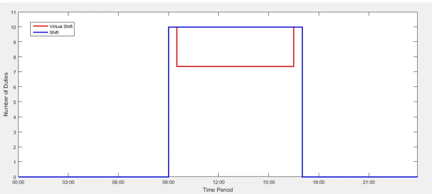
6.1 Virtual Shifts Figure 4: Shift and Virtual Shift
the shift is required to have a total break time of 80 minutes. Taking a time period of 5 minutes, we find that InactiveP eriodsis equal to 14 . Note that the demand fulfilled by the two is equal for the first few and last few time periods of the shift, but the virtual shift has a lower number of active workers in the rest of the periods. This is to account for break time which has to be scheduled.
While finding solutions we noticed that by choosing a lower value for the number of inactive periods we obtained better results. More specifically be usingIP∗ for the inactive periods instead, where
IP∗ =total break time (72)