University of Warwick institutional repository: http://go.warwick.ac.uk/wrap
This paper is made available online in accordance with
publisher policies. Please scroll down to view the document
itself. Please refer to the repository record for this item and our
policy information available from the repository home page for
further information.
To see the final version of this paper please visit the publisher’s website.
Access to the published version may require a subscription.
Author(s): R. Hu, Y. V. Bogdanova, C. J. Owen, C. Foullon, A. N.
Fazakerley, and H. Re`me
Article Title: Cluster observations of the midaltitude cusp under strong
northward interplanetary magnetic field
Year of publication: 2008
Link to published article: http://dx.doi.org/10.1029/2007JA012726
Cluster observations of the midaltitude cusp under strong northward
interplanetary magnetic field
R. Hu,1,2,3Y. V. Bogdanova,1,4C. J. Owen,1C. Foullon,1A. N. Fazakerley,1and H. Re`me5
Received 10 August 2007; revised 31 January 2008; accepted 17 March 2008; published 22 July 2008.
[1] We report on a multispacecraft cusp observation lasting more than 100 min. We
determine the cusp boundary motion and reveal the effect on the cusp size of the interplanetary magnetic field (IMF) changing from southward to northward. The cusp shrinks at the beginning of the IMF rotation and it reexpands at the rate of 0.40° invariant latitude per hour under stable northward IMF. On the basis of plasma signatures inside the cusp, such as counterstreaming electrons with balanced fluxes, we propose that pulsed dual lobe reconnection operates during the time of interest. SC1 and
SC4 observations suggest a long-term regular periodicity of the pulsed dual reconnection, which we estimate to be 1 – 5 min. Further, the distances from the spacecraft to the reconnection site are estimated on the basis of observations from three satellites. The distance determined using SC1 and SC4 observations is 15 RE and that determined from SC3 data is8RE. The large-scale speed of the reconnection site sunward motion is 16 km s1. We observe also a fast motion of the reconnection site by SC1, which provides new information about the transitional phase after the IMF rotation. Finally, a statistical study of the dependency of plasma convection inside the cusp on the IMF clock angle is performed. The relationship between the cusp stagnation, the dual lobe
reconnection process, and the IMF clock angle is discussed.
Citation: Hu, R., Y. V. Bogdanova, C. J. Owen, C. Foullon, A. N. Fazakerley, and H. Re`me (2008), Cluster observations of the midaltitude cusp under strong northward interplanetary magnetic field,J. Geophys. Res.,113, A07S05, doi:10.1029/2007JA012726.
1. Introduction
[2] The cusp regions are null points in the magnetic field above the southern and northern poles and are populated by magnetosheath-like plasma with specific particle signatures. It is now believed that the most common process responsible for the magnetosheath plasma penetration into the magnetosphere is magnetic reconnec-tion. During reconnection between terrestrial magnetic field lines and the interplanetary magnetic field (IMF) lines, new field lines with one end at the Earth and the other end in the interplanetary medium are created. Thus, along such field lines, the solar wind plasma may penetrate into the Earth’s magnetosphere. It is known that recon-nection is more likely to happen at the dayside magneto-pause near the subsolar point during southward IMF [Dungey, 1961], or at locations where the shear between terrestrial field lines and IMF is very large.
[3] During northward IMF, reconnection is more likely to occur poleward of the cusp region, in the lobe sector of the magnetopause [Dungey, 1963; Crooker, 1979]. The signatures of lobe reconnection in cusp observations are: injections of particles at the poleward edge of the cusp; an inverse energy-latitude dispersion in the ion energy-time spectrogram, i.e., the energy of the injected particles increases with increasing latitude; an inverse low-energy ion cutoff observed near the poleward boundary of the cusp [e.g., Reiff et al., 1980; Burch et al., 1980]; and sunward convection inside the cusp [e.g., Smith and Lockwood, 1996]. The cusp formed because of lobe reconnection has often been observed during northward IMF [e.g., Fuselier et al. , 2000a, 2000b; Twitty et al., 2004; Trattner et al., 2004;Lavraud et al., 2005; Bogdanova et al., 2005].
[4] Moreover, it was suggested that during northward IMF, dual lobe reconnection might take place [e.g., Song and Russell, 1992]. During dual lobe reconnection, the open field lines of lobes in both hemispheres reconnect poleward of the cusps with the magnetosheath field lines, thus creating newly closed field lines with magnetosheath plas-ma captured inside them. The signatures of dual lobe reconnection have been reported in the magnetosheath boundary layer [e.g.,Onsager et al., 2001; Lavraud et al., 2006], inside the cusp region at midaltitudes [Fuselier et al., 2001;Bogdanova et al., 2005] and inside the cusp region in the ionosphere [Sandholt et al., 2000;Provan et al., 2005;
Imber et al., 2006]. It has been suggested that signatures of dual lobe reconnection outside the magnetosphere, in the
Here
for
Full Article
1Mullard Space Science Laboratory, University College London, Dorking, UK.
2Ecole Centrale Paris, Paris, France. 3
Now at Tsinghua Centre for Astrophysics, Department of Physics, Tsinghua University, Beijing, China.
4
Now at Department of Physics, La Trobe University, Melbourne, Victoria, Australia.
5Centre d’Etude Spatiale des Rayonnements, Centre National de la Recherche Scientifique, Toulouse, France.
Copyright 2008 by the American Geophysical Union. 0148-0227/08/2007JA012726$09.00
magnetosheath boundary layer, are bidirectional electron beams [e.g., Onsager et al., 2001; Lavraud et al., 2006]. Inside the magnetosphere, a number of signatures have been suggested as features of the reclosed field line configura-tion. Inside the boundary layers the signatures are: (1) the existence of a trapped high-energy plasma sheet population alongside the accelerated magnetosheath-like population and (2) bidirectional electron beams at magnetosheath-like energies with equal fluxes at all energies in the parallel and antiparallel directions [e.g.,Phan et al., 2005].
[5] Inside the cusp region, the signatures of reclosed field lines are (1) a downgoing oxygen population [Fuselier et al., 2001], which might be explained by the ion outflow from the opposite hemisphere (however, such a population is rarely observed because of a large travel time); (2) accelerated plasma population with energies higher than inside the typical cusp, which might be explained by the additional plasma acceleration at the second reconnection site [e.g., Onsager et al., 2001; Bogdanova et al., 2005]; and (3) an isotropic plasma population, which might be explained by pitch angle scattering of the ion and electron populations on field lines with a long history since recon-nection [Bogdanova et al., 2005]. There are various sugges-tions about the expected plasma convection signatures inside the cusp, which correspond to dual lobe reconnection.
Bogdanova et al.[2005] proposed that plasma observed on closed field lines may be almost stagnant, as these field lines are disconnected from the solar wind driver. Conversely,
Provan et al.[2005] andImber et al.[2006] suggested that the process of dual lobe reconnection may be accompanied by a strong sunward convection of plasma. However, convection of reclosed field lines might be more compli-cated: at the beginning, when a field line just undergoes reconnection in the second hemisphere, some sunward convection might be observed. Later, when the reclosed field line ‘‘sinks’’ inside the magnetosphere, the convection is expected to become nearly stagnant. Thus, we suppose that previous studies deal with different ‘‘stages’’ of the lifetime of reclosed field lines. These studies based their conclusions on an investigation of single events. Thus, a wider sample of events needs to be studied in order to understand plasma convection inside the cusp driven by dual lobe reconnection.
[6] The IMF conditions which are favorable for dual lobe reconnection to occur is another area of active debate. On the basis of ionospheric observations, Imber et al. [2006] suggested that dual lobe reconnection might occur only under very strong northward IMF with the magnitude of the clock angle less than 10°. Here, the IMF clock angle is defined as CA = tan1(BY/BZ) whereBYand BZ are components in the GSM coordinate system.
How-ever, on the basis of observations of bidirectional electron beams in the magnetosheath, Lavraud et al. [2006] performed a statistical study which showed that dual lobe reconnection might occur under IMF clock angles in the range ±(0 – 40°). Throughout the paper, we will refer to the clock angle magnitude when we speak about the clock angle.
[7] Thus, there is ambiguity in (1) the plasma convection signatures inside the cusp region corresponding to the dual lobe reconnection and (2) the IMF conditions favorable for the dual lobe reconnection. The aim of the present work is
to try to address these two questions. To do this, we studied midaltitude cusp crossings by Cluster under northward IMF with different clock angles. We found only one event during 1 year of observations (2002) when Cluster crossed the midaltitude cusp region under very strong northward IMF with clock angle <10°. We first studied this event in depth to find unambiguous evidence of the signatures of dual lobe reconnection, assuming that for such IMF conditions dual lobe reconnection does indeed occur. Then we performed analysis of the plasma convection inside the midaltitude cusp region under different clock angles to see if the slow convection inside the cusp is observed for lower clock angles and thus might indicate the occurrence of dual lobe reconnection.
[8] This manuscript is organized as follows: section 2 gives a brief description of the Cluster and ACE missions and the instruments used in this study, section 3 presents Cluster multispacecraft observations of one event under strong northward IMF, section 4 contains discussion of this event, section 5 presents results of statistical study of the plasma convection inside the cusp, and finally section 6 gives the conclusions.
2. Cluster and ACE Satellites and Instrumentation
[9] This study uses data from the Cluster satellites inside the cusp. The Cluster orbit has a perigee of 4 RE, an
apogee of19.7RE, an inclination of90°, and an orbital
period of57 h [Escoubet et al., 2001]. The observations reported here were acquired by the Plasma Electron and Current Experiment (PEACE) [Johnstone et al., 1997], as well as by the Hot Ion Analyzer (HIA) and Composition and Distribution Function (CODIF) sensors, which are parts of the Cluster Ion Spectrometer (CIS) experiment [Re`me et al., 2001]. These instruments are mounted on each of the 4 Cluster satellites. The HIA sensor employs an electrostatic analyzer (ESA) to measure ions of all species with high angular and high-energy resolution. The CODIF sensor combines a top hat analyzer with an instantaneous 360°
field of view, with a time of flight section to measure the complete 3-D distribution functions of the major ion spe-cies, H+, He++, He+, and O+. The sensor covers the energy range between 0.02 and 38 keV/q with a time resolution of 4 s. Each PEACE package consists of two sensors, the HEEA (High-Energy Electron Analyzer) and the LEEA (Low-Energy Electron Analyzer), mounted on diametri-cally opposite sides of the spacecraft. They are designed to measure the 3-D velocity distributions of electrons in the range of 0.6 eV to 26 keV, with a time resolution of 4 s. The spacecraft potential was measured by the Electric Fields and Waves (EFW) instrument [Gustafsson et al., 2001]. We also used magnetic field data from the Fluxgate Magnetometer (FGM) [Balogh et al., 2001] with 4 s resolution.
Proton Alpha Monitor (SWEPAM) [McComas et al., 1998]. The time lag associated with solar wind convection between the ACE and Cluster observations inside the cusp was calculated on the basis of theXcomponent of the solar wind velocity in the GSE coordinate system (measured with a resolution of 64 s) and the position of ACE along Sun-Earth line (GSEXaxis).
3. Observations of the Midaltitude Cusp Crossing During Strong Northward IMF
3.1. Cluster Orbit, IMF, and Solar Wind Conditions
[11] During September 2002 the Cluster satellites crossed the midaltitude cusp region in the string-of-pearls configu-ration. In this formation, Cluster SC3 is separated from the other three spacecraft by up to2.5REwhen it is inside the
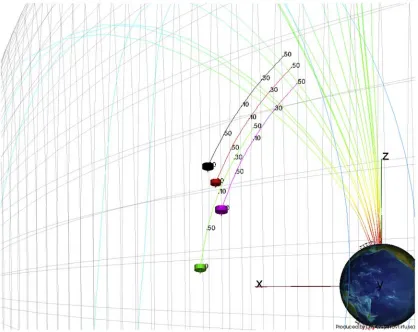
midaltitude cusp and polar cap. On 8 September 2002 during the period 0450 – 0640 UT, the Cluster satellites cross the northern cusp region. The orbits of four Cluster satellites moving from low to high latitudes via the cusp are shown in Figure 1, with SC1 indicated by black, SC2 by red, SC3 by green, and SC4 by magenta. The order of the passage through the cusp is SC1, SC2, SC4, and SC3. In this paper we will concentrate on observations from SC1,
SC3, and SC4 in order to explore the full data set available from these three satellites.
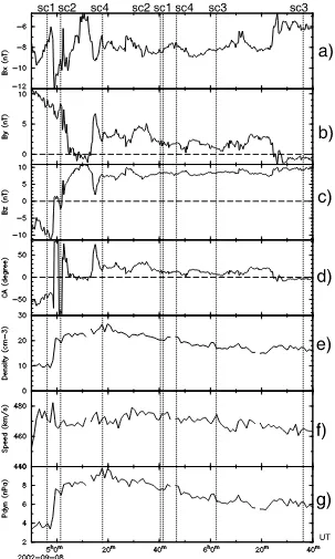
[12] The IMF and the solar wind (SW) conditions, observed by the ACE spacecraft between 0450 and 0640 UT, are shown in Figure 2. Figures 2a – 2c show the GSMX,Y, andZcomponents of the IMF; Figure 2d shows the clock angle (CA) of the IMF; Figure 2e presents the H+density of the solar wind; Figure 2f shows the bulk speed of the solar wind; and the Figure 2g shows the dynamic pressure of the solar wind. The time series are shifted forward by 55 min. This propagation delay is estimated by taking into account theX component of the solar wind velocity, 460 – 480 km s1during the event and theXGSE location of the ACE satellite. This time lag is consistent with the time lag calculated using a recent method discussed byWeimer et al.
[2003]. The eight vertical dashed lines correspond to the times when each Cluster satellite enters and leaves the cusp region.
[13] At the beginning of the interval of interest, when SC1 and SC2 enter the cusp, the IMF is southward (BZ 5 to 10 nT) and largely duskward (BY 5 – 10 nT).
[image:4.612.98.516.59.391.2]From0457 to0503 UT, the solar wind dynamic pressure increases from 4 to 8 nPa, and the IMF turns northward then remains strongly northward (BZ8 – 10 nT) until the end of Figure 1. Orbits of Cluster satellites in the GSMX-Zplane during the period 0430 – 0600 UT. The black
the period of interest, when SC4 and SC3 enter and leave the cusp region. The density of the solar wind reaches its highest value, 27 cm3 at 0520 UT, then gradually decreases and returns to a stable value of 16 cm3. The solar wind pressure also reaches its highest value of 10 nPa at 0520 UT. The IMF is due northward, CA 0°, from
0505 to0513 UT; from0517 UT the IMF CA remains <±20°. For the whole period, the IMF BX component is
negative; this favors the occurrence of reconnection in the northern lobe sector (summer hemisphere).
[image:5.612.155.458.56.561.2][14] In the next section we report the data from SC1, SC4, and SC3, in this order the satellites crossing successively the cusp, and report in detail the azimuthal cuts through the electron energy spectra and ion phase space density distributions for the selected times. Further
discussion will be in the GSM coordinate system unless otherwise stated.
3.2. Cusp Crossing Observations by Cluster 1
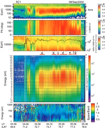
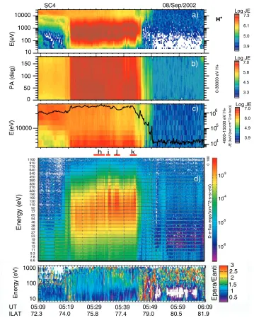
[15] An overview of SC1 plasma data is shown in Figures 3 and 4. Figure 3 presents electron and ion data
[image:6.612.129.485.56.487.2]based on the CIS-HIA and PEACE LEEA sensor obser-vations on 8 September 2002 from 0446 to 0546 UT. Figures 3a and 3b present the ion energy-time spectrogram and pitch angle distribution measured by CIS-HIA instru-ment. The whole energy range of the instrument has been used for Figures 3a and 3b. Differential energy flux is
color coded. Figure 3c shows the energy-time spectro-gram of the ions for the high-energy population only,
E= 4 – 32 keV (corresponding scale on the left). Differential energy flux is color coded. The over-plotted black line represents the integrated energy flux of ions with energies
E = 4 – 15 keV (corresponding scale on the right). This limited energy range is used in order to include the accelerated magnetosheath population and exclude the plas-ma sheet population. Figure 3d consists of 30 sections, where each section shows the electron pitch angle spectro-gram for an energy range indicated on the left. The 4 s data from the PEACE LEEA sensor have been used. The
spacecraft potential has been used to eliminate photoelec-trons, and the energy of the population has been corrected for this effect. Differential energy flux is color coded. Figure 3e is an energy-time plot where the anisotropy of the counterstreaming electron population is color coded. The color represents the ratio of the differential energy flux of the population moving parallel to the magnetic field to the differential energy flux of the population moving antiparal-lel to the magnetic field. Below the plot, the universal time and corresponding invariant latitude are indicated. The short bold lines it the middle indicate the times of the separate electron beams a – g discussed in the text.
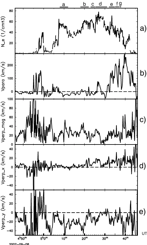
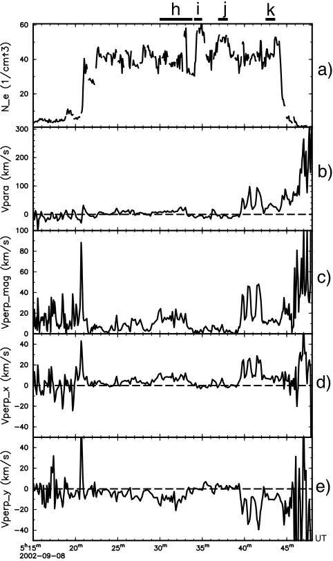
[16] Figure 4 shows the plasma moments calculated on the basis of the PEACE and CIS-HIA observations on SC1 on 8 September 2002 from 0446 to 0546 UT. Figure 4a presents the electron density and Figures 4b – 4e show the ion bulk velocity in the magnetic field-aligned coordinate system: the velocity parallel to the magnetic field (Figure 4b), the magnitude of the convection (perpendicular to the magnetic field) velocity (Figure 4c), the X and Y
components of the perpendicular velocity (Figures 4d and 4e, respectively). The GSM coordinate system has been used for the velocity components. The short bold lines above the plot indicate the times corresponding to the separate electron beams a – g discussed in the text. We use the ion velocity perpendicular to the magnetic field lines to demonstrate the motion of the field lines, because of the validity of ‘‘frozen in’’ conditions. Therefore we consider only the perpendicular velocity for the plasma convection further in this paper.
[17] From 0456 UT SC1 begins to detect magneto-sheath-like plasma, e.g., ions with energy in the range 100 eV – 6 keV (Figure 3). From0457 to0500 UT the spacecraft detects a significant flux enhancement of both electrons and ions. During this period we observe three short durations separated electron beams whose energy ranges from 14 to 270 eV, at 0457, 0459, and
0500 UT. Both downgoing and upgoing populations are seen, while the upgoing population (pitch angle 180°) seems to dominate the low-energy (9.6 eV) and high-energy (290 eV) bands. Further, the ion spectrogram (Figure 3a) shows the low-energy cutoff decrease with time and lati-tude, which is expected during dayside reconnection events [e.g., Smith and Lockwood, 1996]. The ions are observed over an energy range from 300 eV to 4 keV, while at
0500 UT, they appear over an energy range from 200 eV to 3 keV. During this time, the ion parallel velocity is positive, with magnitude up to 100 km s1, which indicates a significant downward ion injection. Meanwhile, the per-pendicular velocity (Figures 4d and 4e) shows duskward convection, and the sunward-antisunward component of the convection is highly variable.
[18] From0500 to0504 UT, the high-density popula-tion disappears except for one weak beam which is seen at
[image:7.612.60.301.56.457.2]0501 UT. At this time plasma sheet ions are evident. However, the electrons are still of magnetosheath origin, with energies 9.3 – 260 eV. Such plasma characteristics are typical for the electron edge of the low-latitude boundary layer [Bogdanova et al., 2006]. We note that these variations in plasma parameters appear when the solar wind dynamic pressure strongly increases, and thus it might be a spatial rather than temporal variation of the plasma parameters.
[19] Later, the electron density increases quickly from 20 cm3 at 0504 UT to 60 cm3 at 0507 UT. From
0504 to 0508 UT, the electron and ions distributions show also an energy-latitude dispersion decreasing with latitude, indicating that these populations may surely be on field lines which have undergone dayside reconnection. From 0508 to 0542 UT, we observe seven separate strong electron beams (Figure 3d) which correspond to the peaks of the electron density as shown in Figure 4, at 0508 – 0512 UT (beam a), 0518 – 0522 UT (beam b), 0523 – 0525 UT (beam c), 0525 – 0531 UT (beam d), 0532 – 0535 UT (beam e), 0535 – 0537 UT (beam f), and 0537– 0538 UT (beam g). These separate electron beams, which might be identified as separate variations in the electron energy, flux and density, are indicated by bold horizontal lines in the middle of Figure 3 and on the top of Figure 4.
[20] There are other electron populations apart from these beams, but with lower-energy flux and density. Beam d has the highest density (Figure 4a). Beam a has electron energy from 9.6 to290 eV (Figure 3d). Significant fluxes of high-energy (340 eV) population are observed in beams b, d, e, f, and g. We note that beams b, d, and e seem to be bidirectional in all energy channels, including the high-energy end, while the upgoing population dominates the high-energy end of beams f and g. Equal fluxes of the counterstreaming population during beams b, d, and e and dominant upgoing population at high energies during beams f and g also can be seen in Figure 3e. In Figure 3e, if we compare the ratio of parallel fluxes and antiparallel fluxes during the electron beams and near the cusp equatorward and poleward boundary, it is clear that the electron beams are more balanced. Beam c does not have a population in the 340 eV band, but it seems to be bidirectional in all energy channels. From 0530 UT, the low-energy cutoffs of the beams increase with latitude, which indicates lobe reconnection events [Reiff et al., 1980;Burch et al., 1980;
Twitty et al., 2004].
[21] We now look into the ion spectrogram and convection during the same time period. From0508 to0542 UT, we observe a general inverse ion low-energy cutoff, e.g., the ion low-energy cutoff is increasing with latitude (or, in our case, time) in the ion spectrogram (Figure 3a), which is consistent with lobe reconnection. Some short-scale decreases of the low-energy cutoff are observed from0530 UT. This may relate to the motion of the cusp, or to the separate plasma injections in the cusp [Lockwood and Smith, 1994]. Investi-gating only the high-energy part of the ion population (Figure 3c), we observe enhanced fluxes of high-energy ions (E> 4 keV) at 0456 – 0500 UT, 0505 – 0512 UT (including the time interval of beam a), 0517 – 0523 UT (around the time of beam b), 0524 – 0528 UT (beams c and d), and 0530 – 0542 UT (beams d, e, f, and g). We note that the enhance-ments of high-energy ion fluxes,E = 4 – 15 keV, generally correlate with the electron beams taking into account the fact that the ions and electrons have different travel times. Moreover, during some short time intervals, enhancements of the fluxes of ions with plasma sheet energies, E = 20 – 38 keV, are detected.
[22] From0507 to0532 UT (beams a, b, c, and d), the pitch angle distribution of ions remains isotropic. During this time interval the parallel velocity is low,Vpara– 0 – 40 km s1, which corresponds to domination of the upflowing
population. However, during the small time intervals inside beams b, c, and d, the parallel velocity becomes positive,
Vpara = 0 – 40 km s1, indicating domination of plasma injections. During the time interval 0507 – 0532 UT, the perpendicular velocity is relatively small (jVperpj < 40 km s1). Plasma convection in the sunward-antisunward direction is very low,Vperp_x0 – 20 km s1, while stronger
convection is observed toward dawn,Vperp_y – 0 – 40 km
s1. We consider this region to be a region with reduced convection because much lower convection speeds are observed in comparison with the convection detected near the cusp poleward boundary. Thus, from 0532 UT, the plasma moves significantly sunward and dawnward, with
Vperp_x 20 – 40 and Vperp_y – 0 – 60 km s1. From 0532 to 0542 UT, downgoing ion injections dominate, except for short periods around 0536 (beam f) and 0538 UT (beam g), where the isotropic distribution reappears. Very high parallel velocities (Figure 4b) also indicate ion injec-tions from0532 UT, withVparaup to 300 km s1. We note that this downgoing injection appears at the poleward boundary of the cusp, which is consistent with the lobe reconnection process. After0542 UT, before entering the polar cap, the spacecraft detects low fluxes of magneto-sheath-like ions and electrons. This might indicate some boundary layer population.
[23] To summarize, SC1 enters the cusp when the IMF changes orientation from southward to northward. The spacecraft detects a region with reduced convection in the middle of the cusp and plasma injections with inverse low-energy cutoff near the poleward boundary of the cusp, which is consistent with lobe reconnection. Several separate electron beams are observed, and some of them are bidi-rectional at all energies. On the cusp equatorward boundary, a short-term separate population consistent with dayside reconnection is observed. We will discuss these plasma properties later on in the paper.
3.3. Cusp Crossing Observations by Cluster 4
[24] An overview of the SC4 plasma data is shown in Figures 5 and 6 whose formats are similar to Figures 3 and 4, respectively. However, for the analysis of ion data we used observations of the H+ ion population from the CIS-CODIF instrument, as the HIA instrument does not work on SC4. In this case we use high-resolution ground-calculated 3-D moments to produce the electron density shown in Figure 6 since the PEACE instrument is in burst mode on SC4.
[25] From 0519 UT SC4 begins to detect magneto-sheath-like plasma about 16 min after SC1. In both electron and H+ spectrograms we can see clear sharp equatorward and poleward boundaries of the cusp, at 0521 and
0546 UT, respectively. During this cusp crossing, many electron beams are seen, and some of them are bidirectional in all energy channels. Before0530 UT, the electron energy ranges from 14 to 220 eV. From0530 UT, higher-energy electrons (about 280 eV) are detected as well, and the lower-energy (about 14 and 19 eV) population declines. After
spectrogram of H+ ions, we observe reversed energy-time dispersion from0530 UT. The reverse low-energy cutoff is observed from0515 UT. It is also interesting to note that the ion population detected on SC4 is ‘‘broader’’ in comparison with the population observed on SC1. Thus, energies of magnetosheath-like H+ ions detected on SC4 are E = 30– 10000 eV (Figure 5a). High-energy ions (E = 4 – 15 keV) are detected generally throughout the cusp crossing, however it is possible to see some particular flux enhancements before 0535 UT (beams h and i) and 0536– 0537 UT and 0539– 0544 UT (beam k). The spikes of magnetosheath-like ion population with additional high fluxes at high energies corre-spond partially to the electron beams. Additionally, significant fluxes of ions with plasma sheet energies are detected during this cusp crossing, especially during the interval 0519 – 0535 UT. However, we should note that the CIS-CODIF instrument saturates in high-density plasma, and thus such
strong ion fluxes observed on SC4, especially at high energies, can be partially due to saturation effects.
[26] From0521 UT to0539 UT, the parallel velocity is very low, Vpara = ±20 km s1 and the perpendicular velocity is less than 20 km s1, with convection being slightly sunward, Vperp_x = 0 – 10 km s1, and mostly
dawnward, Vperp_y varies from 5 to 20 km s1. Thus,
convection is much lower than that observed inside the cusp by SC1. We can consider this part of the cusp as being nearly stagnant. The ions inside the cusp are isotropic, which also indicates a nearly stagnant cusp. From
0539 UT, the plasma injections are evident, with Vpara= 50 – 200 km s1. The pitch angle spectrogram shows that the downgoing population slightly dominates. At this time, the plasma moves sunward, Vperp_x = 20 – 60 km s1, and
[image:9.612.131.490.55.504.2]dawnward, Vperp_y varies from 0 to 50 km s1. We Figure 5. Electron and ion data based on the PEACE LEEA and CIS-CODIF observations on SC4 on
observe ion injections at the poleward boundary of the cusp, which is again a signature of lobe reconnection.
[27] To summarize, SC4 crosses the cusp during the period when the IMF remains strongly northward. SC4 detects some plasma properties similar to the SC1 observa-tions inside the cusp; especially, the bidirectional electron beams with similar parallel and antiparallel fluxes at all energies in the nearly stagnant cusp region are commonly observed. These beams are observed simultaneously with an increase of ion fluxes with energies 4 keV < E < 10 keV. However, the convection inside the cusp observed by SC4 is lower than that observed by SC1.
3.4. Cusp Crossing Observations by Cluster 3
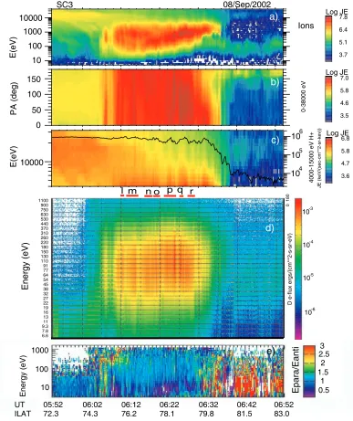
[28] An overview of the SC3 plasma data is shown in Figures 7 and 8 whose formats are again similar to Figures 3
and 4, respectively. Before0605 UT, SC3 is in the dayside plasma sheet, characterized by high-energy ion population (Figure 7a). From 0604 UT SC3 begins to detect the magnetosheath-like ions with energy ranged from 80 to 400 eV about 64 min after SC1. From 0605 UT, the population of magnetosheath-like ions is enhanced, and their energy band broadens to 20 – 2000 eV. During this period, the ion spectrogram shows low-energy cutoff decreasing with latitude. The peak of injection is detected from 0605 to 0606 UT. Then the fluxes reduce until
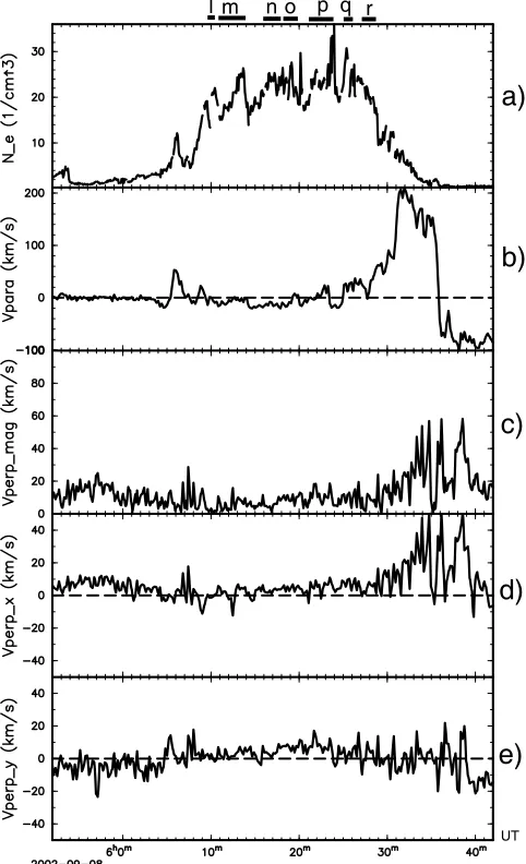
0608 UT. From0608 UT, the ion fluxes are significantly enhanced and remain high until the end of the cusp crossing. From 0604 to 0607 UT, the plasma sheet-like ions with energies between 8 and 38 keV are still seen (Figures 7a and 7b). Figure 8b shows a net parallel flow between0605 and 0607 UT withVpara= 0 – 60 km s1, which indicates plasma injections. The plasma convection defined by the perpen-dicular velocity is weak (Vperp < 15 km s1). The X component of the perpendicular velocity ranges between 0 and2 km s1from 0604 to 0606 UT (which is zero in the error range), and it becomes variable between ±15 km s1 from 0606 to 0610 UT (Figure 8c). TheYcomponent of the perpendicular velocity changes its direction at about 0605 UT and reaches its maximum value of 15 km s1 (Figure 8e). Before 0605 UT, dawnward convection domi-nates, while after 0605 UT, duskward convection dominates. As the convection velocity is very low, we may also refer this period as stagnation. The electron density presented in Figure 8a also shows a separate injection between 0605 and 0607 UT. A nearly bidirectional electron beam is detected at
0606 UT (Figures 7d and 7e), with energy ranging from 25 to 260 eV. During the interval 0606 – 0608 UT, the reduced fluxes of the magnetosheath-like electrons are detected.
[image:10.612.61.302.58.464.2][29] From0608 UT, magnetosheath-like electrons with normal fluxes are continuously detected. Generally elec-trons inside this cusp crossing are not isotropic. The intensity of the electron fluxes is variable, mainly in the energy range 22 – 440 eV, and dominated by an upgoing (pitch angle180°) population (Figure 7d). For the energy range 20 – 41 eV, the electrons are also mainly upgoing. Figure 8a shows several peaks in the electron density, at 20 – 30 cm3, which indicates the multiple injections of electrons. We can identify these electron beams at
0610 UT (beam l), 0611 – 0614 UT (beam m), 0616 – 0618 UT (beam n), 0618– 0620 UT (beam o), 0621 – 0624 UT (beam p), 0625 – 0626 UT (beam q), and 0627 – 0629 UT (beam r). For all these beams, the upgoing population dominates in the energy band 14 – 310 eV (Figures 7d and 7e). However, beams o, p, and q are much more populated in the energy band around 280 eV and still populated in the energy band around 430 eV. Moreover, at the high-energy end (280 eV), these beams are nearly bidirectional. The time periods of electron beams n, o, p, q, and r correlate very well with observed enhancements of the fluxes of the high-energy part of the magnetosheath-like population (Figure 7c). [30] During the interval 0610 to 0625 UT, the ion parallel velocity is very low, Vpara = ±20 km s1. The X component of the convection velocity remains less than 10 km s1and theYcomponent remains less than 15 km s1. Despite the low speed the convection keeps mainly sunward and duskward, consistent with the expectation of lobe reconnection under negative IMFBY. We refer to this region Figure 6. The plasma parameters calculated on the basis
as the nearly stagnant cusp, because the convection velocity is much lower than that observed near the poleward bound-ary, where the X component of the convection velocity is
10 – 50 km s1.
[31] Between 0625 and 0640 UT, Cluster SC3 moves from the cusp into the northern lobe region, and crosses the poleward boundary of the midaltitude cusp at 0636 UT. This region is characterized by the appearance of strong downgoing magnetosheath-like ion injections (Figure 7b), high fluxes of short-duration electron beams (Figure 7d), net field-aligned flow, Vpara 20 – 200 km s1, and strong sunward convection, Vperp_x = 10 – 50 km s1 (Figures 8b
and 8d). The ion spectrogram shows a clear low-energy cutoff at the poleward boundary of the cusp and reversed energy-time dispersion, which are again signatures of the
lobe reconnection process [e.g.,Reiff et al., 1980;Burch et al., 1980; Smith and Lockwood, 1996]. Plasma convection past the spacecraft is mainly sunward with theXcomponent of the perpendicular velocity remaining positive and vary-ing up to 50 km s1. TheYcomponent of the perpendicular velocity is highly variable between 20 and 20 km s1. From 0636 UT, SC3 leaves the cusp and moves into the lobe region of the magnetosphere.
[32] To summarize, SC3 enters the cusp when the IMF has remained strongly northward (IMF clock angle
[image:11.612.117.504.58.519.2]0 – 20°) for more than 1 h. SC3 detects a separate population on the cusp equatorward boundary, a nearly stagnant part in the middle, and the features of lobe injection near the poleward boundary. Electron beams in the nearly
stagnant cusp region are also observed, but they are not completely bidirectional.
3.5. Azimuthal Cuts Through the Electron Energy Spectra and Ion Phase Space Density Distributions
[33] The above observations show that the Cluster satel-lites detect high-energy electron and ion fluxes for some periods during the cusp crossing. Some of the electron beams seem to be nearly bidirectional on the electron spectrogram. We examine the electron azimuthal cuts through the electron energy spectra and ion phase space density distributions, which may provide detailed informa-tion on the plasma characteristics observed by the three spacecraft. We look into electron azimuthal cuts of differ-ential energy flux and ion distribution functions every 1 min during the cusp crossing. During the periods having the high-energy electron fluxes, and additionally accelerated
ions, we examine electron energy spectra every 4 s (spin resolution) and the ion distribution functions every 20 s. These time selections are based on the assumption that the electrons maybe highly variable and the spectra may change significantly within 4 s. Contrary, the ions are heavier and thus the timescale can be larger.
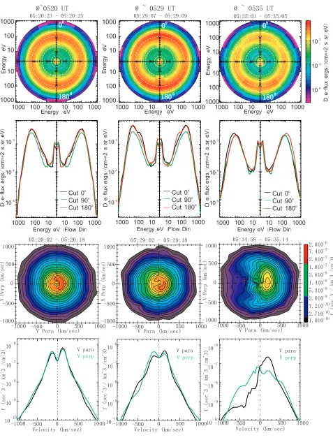
[34] Some results of our study are shown in Figures 9, 10, and 11 which correspond to observations from SC1, SC4, and SC3, respectively. Figures 9, 10, and 11 all have a similar format and show electron azimuthal cuts through the electron energy spectra and H+ phase space density distri-butions based on the PEACE LEEA and CIS-CODIF observations for the particular time intervals indicated above each column. The first row shows the electron 2-D azimuthal cuts of the electron spectra in the differential energy flux units, in which 0°(top) indicates the direction parallel to the local magnetic field, and 180° (bottom) indicates the direction antiparallel to the local magnetic field. The differential energy flux is color coded, and the same scale has been used for all columns. The second row shows the cross sections of the 2-D cuts in the parallel, perpendicular and antiparallel directions. The right half of the plot corresponds to particles flowing in the direction of the chosen cut angle, thus the black line corresponds to 0°
pitch angle particles, the green line corresponds to 90°pitch angle particles and the red line corresponds to 180° par-ticles. The left half of the plot corresponds to particles traveling in the opposite direction of the chosen cut angle. Thus, the legend is reversed for this part of the plot, i.e., the black line corresponds to 180°pitch angle particles, the green line corresponds to 90°pitch angle particles and the red line corresponds to 0°particles. The third row presents the 2-D cross sections of the H+ion distribution functions in a plane containing (Vpara, Vperp). Vpara is aligned with the local magnetic field, and Vperp is in the (V B) B direction. The colors represent the phase space density. Contours are evenly spaced logarithmically between the minimum and maximum values. The same scale has been used for all columns. Vpara > 0 corresponds to the down-going population andVpara< 0 corresponds to the upgoing population. The fourth row shows the 1-D cross sections of the H+ ion distribution along the magnetic field direction (Vperp = 0, black line) and perpendicular to the magnetic field direction (Vpara = 0, green line).
[35] In the SC1 observations we note that beams b and d have high-energy electrons and accelerated ions. We com-pare plasma properties during beams b and d with those during beams f and g near the cusp poleward boundary. Figure 9 shows three electron azimuthal cuts through the electron energy spectra and ion phase space density distri-butions from SC1: one example (0520 UT) for beam b, one example (0529 UT) for beam d, and one example (0535 UT) for beam f. The 1-D cross sections of the electron 2-D cuts (second row) indicate that at0520 UT and
[image:12.612.61.302.60.456.2]0529 UT the fluxes of parallel and antiparallel populations are generally higher than the perpendicular populations for energies below 500 eV. Above 500 eV, the fluxes in the parallel, antiparallel and perpendicular directions are nearly equal. Additionally the parallel and antiparallel populations have very well balanced fluxes for energies above 40 eV. For the low-energy (10 – 40 eV) bin, the antiparallel electron flux exceeds the parallel one. Contrary, at0535 UT, near
the poleward boundary of the cusp, the upgoing electron population with energies above100 eV is dominant, and counterstreaming populations are not balanced. Above 500 eV, the fluxes of the perpendicular population are nearly equal to the fluxes of parallel and antiparallel populations. In the ion distributions, at 0520 and
0529 UT, along the presumably reclosed field lines, we observe nearly isotropic ion distribution, with some enhancement of downgoing fluxes. At the same moments, the parallel and perpendicular 1-D cuts of the ion population are similar, also indicating that ions are quasi-isotropic. At 0535 UT, near the poleward boundary we observe a D-shaped ion distribution. The downgoing ion population clearly dominates, which indicates the ongoing plasma injections at this time. Comparison of 1-D cuts of the ion population at this time shows that the perpendicular velocity is higher than the bulk parallel velocity of the upgoing population.
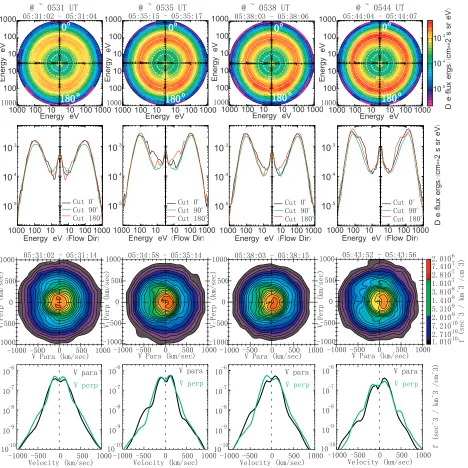
[36] Similar observations are presented for SC4 in Figure 10. Beams h, i, and j have high-energy electrons and accelerated ions. We show three examples (0531 UT (inside beam h),0535 UT (inside beam i), and0538 UT (inside beam j)) for these beams, as well as one example (0544 UT) near the poleward boundary of the cusp. As one can see, inside beam h, fluxes of counterstreaming electrons are very well balanced at nearly all energies. Inside beams i and j fluxes of counterstreaming electrons are balanced for higher energies, above100 eV. For the population with energies 100 eV (near mean energy), there are some small disagreements between fluxes of downgoing and upgoing populations. This disagreement gets larger for energies less than 40 eV. Thus, it is possible to conclude that for beams i and j the electron population is bidirectional with nearly equal fluxes at energies above 40 eV. Near the poleward boundary (Figure 10 fourth column), we observe dominant parallel population at ener-gies above 70 eV and dominant antiparallel population at energies below 70 eV. Thus, this population is strongly unbalanced. We also should note that the electron spectra are very variable throughout the cusp and small changes are seen every spin. Thus, the ideal situation when the counter-streaming electron population is completely balanced at all
energies is rarely seen. The presented electron spectra during beams i and j are more typical, when there is a good balance for the high-energy electron population,E> 100 eV, and there are some small disagreements between bidirec-tional fluxes at 70 – 110 eV. In the ion distributions, we observe, similar to the SC1 case, nearly isotropic ions inside beams h, i, and j, along the presumably reclosed field lines. Near the poleward boundary of the cusp, more anisotropic ion population is seen.
[37] We analyze electron and ion data in the same way for SC3. Beams o, p, and q have high-energy electrons and accelerated ions. In Figure 11, we show four examples for each beam o (0619 UT), p (0623 UT), q (0625 UT), and r (0627 UT), as well as one example (0631 UT) near the poleward boundary of the cusp. From the electron pitch angle spectrogram (Figure 7d) it is clear that at lower energies, upgoing electrons dominate. Domination of the upgoing electrons at low energies is also evident from the presented electron spectra. Thus, fluxes of the counter-streaming electrons are unbalanced at energies 20 – 200 eV. However, for the examples during beams o, p, and q we observe the bidirectional properties at high energies, above
200 eV. For these events the fluxes of parallel and antiparallel populations with energies above 200 eV are nearly equal. For the example near the poleward boundary, we observe the dominant parallel injections at some energies, E 200 – 900 eV. The similar domination of downgoing electrons with energies 200 – 1000 eV is observed at 0628 UT, inside beam r. The ion distribution functions detected on SC3 are significantly different to those observed by SC1 and SC4. Indeed, we do not observe isotropic distributions in this case. Along the presumably reclosed field lines, when the electron counterstreaming population has nearly equal fluxes in the parallel and antiparallel directions for high-energy part of population, the ion distri-butions are D-shaped and show clear positive and negative low-velocity cutoffs.
3.6. Ion Distribution Near the Equatorward Boundary Observed on SC3
[38] To investigate this anisotropic ion population observed on SC3 further, we study the ion distribution
Figure 9. Electron azimuthal cuts through the electron energy spectra and H+phase space density distributions based on the PEACE LEEA and CIS-CODIF observations on SC1 on 8 September 2002 at0520 (beam b),0529 (beam d), and
0535 UT (near the cusp poleward boundary). The first row shows the electron 2-D azimuthal cuts of the electron spectra in the differential energy flux units, in which 0° indicates direction parallel to the local magnetic field (top) and 180°
functions near the equatorward boundary of the cusp in more detail. We examine the ion distributions every 4 s (the basic time resolution) between 0604 and 0608 UT. We find two subintervals with different ion properties. Examples of these subintervals are illustrated in Figure 12. Each column shows a 4 s ion velocity distribution at one of the subintervals and the time interval is indicated on the top of the column. The first row shows the 2-D cuts of the ion distribution function parallel and perpendicular to the local magnetic field. The phase space density is color coded. The second row shows the 1-D cross sections of the H+ ion distribution at Vperp = 0 (black line) andVpara= 0 (green line).
[39] From 0604 to 0605 UT (Figure 12 left), the distri-butions have mainly three characteristics: a lack of a
[image:15.612.75.543.55.523.2]mirrored ion population (there is no D-shaped population for the negative parallel velocity); a high-energy downgoing population and two positive low-velocity cutoffs. Thus this period is dominated by the downgoing injections. However, it seems that there are two parts in the positive D-shaped downgoing population. The low-energy population is D shaped, whoseVparaandVperpare below 200 km s1, while the high-energy population for Vpara > 400 and Vperp > 400 km s1, which is clear and separated, shows again typical D shaped and implies injection of ions with very high energy. From the cross section at Vperp= 0, several positive parallel velocity cutoffs can be identified (in the downgoing population). The first cutoff is about 80 km s1, and the second is about 200 km s1. Sometimes a third cutoff can also be
Figure 10. The azimuthal cut through the electron energy spectra and H+ phase space density distributions based on the PEACE LEEA and CIS-CODIF observations on SC4 on 8 September 2002 at
Figur
e
1
[image:16.612.62.549.69.702.2]seen (300 – 400 km s1). Each low-velocity cutoff might indicate an independent injection, so there are several independent injections in this period on the same field line. [40] In the second subinterval, from 0605 UT, the mirror ion population appears, as shown in Figure 12 (right). The negative low-velocity cutoff appearing in this period is between 400 and 600 km s1. The high-energy population mixes with the low-energy population and forms one D-shaped population in the downgoing particles. The second and third velocity cutoffs gradually decrease, until
0608 UT, when they could not be discerned in the cross sections anymore.
[41] In summary, ion distributions observed by SC3 show the following special features (Figures 11 and 12):
[42] 1. Dominant downgoing ions. Two distinct D-shaped distributions are observed near the equatorward boundary of
the cusp and one D-shaped distribution is commonly observed through the rest of the cusp.
[43] 2. Several upgoing ion populations near the equator-ward boundary. There are usually two mirrored populations, and two low-velocity cutoffs on the cross section atVperp= 0. These features require further investigation.
[44] 3. On the cusp poleward boundary, we observe the usual lobe reconnection precipitating features.
4. Interpretation and Discussion
4.1. Four Spacecraft Comparison and Cusp Size Variations
[45] Now we compare the observations by the four Cluster spacecraft. For the SC2 observations, we use data from the PEACE experiment only. Because of high
Figure 11. The azimuthal cuts through the electron energy spectra (differential energy flux is color coded) and H+ distribution functions (phase space density is color coded) based on the PEACE LEEA and CIS-CODIF observations on SC3 on 8 September 2002 at0618 UT (beam o),0623 UT (beam p),0625 UT (beam q),0628 UT (beam r), and
[image:17.612.72.543.52.426.2]0631 UT (near the cusp poleward boundary). Same format as Figure 9.
telemetry rate on SC2, we can calculate plasma parame-ters (density and velocity) using 3-D data available with high time resolution. Figure 13 presents a combined plot of the plasma parameters calculated on the basis of the PEACE and CIS observations on four Cluster satellites on 8 September 2002. Figure 13a presents the electron density
with 4 s resolution and Figures 13b – 13d show the ion bulk velocity in the magnetic field-aligned coordinate system: the parallel velocity (b), and the X and Y components of the perpendicular velocity (Figures 13c and 13d, respectively). The GSM coordinate system has been used for the velocity components. For the density estimation the electron data have been used from all four spacecraft. For the velocity estimation the CIS-HIA observations have been used from SC1 and SC3, the CIS-CODIF observations from SC4 (averaged over 30 s), and the PEACE observations from SC2 (averaged over 30 s). The Cluster color code has been used: SC1 is black, SC2 is red, SC3 is green, and SC4 is blue. For better comparison, the time series of SC2 are shifted backward by 5 min, the time series of SC4 are shifted backward by 16 min, and the time series of SC3 are shifted backward by 64 min. The time shifts are calculated from the comparison of the times of the cross-ings of the equatorward boundary of the cusp by the different spacecraft.
[46] We observe clearly different density levels during the four cusp crossing events. We cross checked the electron density from the PEACE instrument with the ion density from the CIS-HIA instrument, and we also cross checked the different PEACE products (3DR, SPINPAD and onboard). All densities agree with each other very well, hence the significance difference in the plasma density between the cusp crossings is not due to calibration errors. SC1 detects the densest plasma; the maximum density observed on SC1 is
80 cm3. Plasma density variations observed on SC2 are very similar to those on SC1, especially during the first 15 min of the cusp crossing. Having in mind that these two satellites are very close to each other, with a time difference of 5 min, we suggest that SC1 and SC2 cross the same plasma population, at least at the beginning of the cusp crossing. However, one special feature observed by SC1 is a separate density peak near the equatorward boundary of the cusp which corresponds to the separate population observed in the electron and ion spectrograms. Comparison of the densities suggests some similarity of the cusp structures during the SC1, SC2, and SC4 crossings. These spacecraft see a sudden outset of the dense plasma; the density tends to maintain the same level in the middle of the cusp; and the density increases significantly in several intervals near the poleward boundary of the cusp. However, SC4 observes a less dense plasma than previous two satellites and variations in the density are not very well related to variations observed by SC1 and SC2. The durations of the injections near the poleward boundary are different: SC1 observes these over a period of 15 min, SC2 for 10 min, SC4 for 7 min, and SC3 for 10 min.
[47] The most dramatic difference in the plasma density is detected on SC3. Indeed, the plasma density inside the cusp appears to decrease during the period of interest by a factor of 3 (from 60 to 20 cm3). This phenomenon is correlated to the density variation of the solar wind. From
[image:18.612.61.302.56.444.2]0520 to 0640 UT, the solar wind density decreases by 38% (Figure 2e). The decrease of the plasma density inside the cusp is also correlated with the IMF being northward for more than 1 h. The statistical study of the cusp density agrees with our observations: it was shown that the cusp density is lower under northward IMF than under southward IMF (F. Pitout, private communication, 2007). We suggest
that the difference in the density may not only be due to the solar wind effect, but may also be the result of a different effectiveness of reconnection processes during southward and northward IMF conditions. The other possible expla-nation can be that during this time interval the cusp moves in the longitudinal direction and SC3 crosses different part of the cusp, probably toward the edge. However, the IMF BY component, which is responsible for the cusp longitu-dinal motion [e.g.,Zhou et al., 2000], is relatively stable at
+2 nT. Thus, we would not expect significant cusp motion in the longitudinal direction during this interval.
[48] The plasma parallel velocities observed on the four spacecraft show similar behavior: the parallel velocity is very low, ±20 km s1, near the equatorward boundary and inside the center of the cusp, and it becomes strong and positive toward the poleward boundary of the cusp, reach-ing 200 – 300 km s1. We also observe some interesting features from the comparison of the convection speeds. During each cusp crossing, we observe a region of very low sunward convection, which we identify as the ‘‘nearly stagnant cusp’’ or ‘‘part of the cusp with reduced convec-tion.’’ Although the cusp crossing durations are conspicu-ously different, the duration of the nearly stagnant cusp crossing is always about 15 min. We note that inside the nearly stagnant cusp, the density variation from SC1 to SC3 is lower (from 40 to 20 cm3), and consistent with solar wind density variations. That suggests the nearly stagnant cusp is one stable region which is less affected by the convection near the boundaries of the cusp. We also note that inside the nearly stagnant cusp (or cusp region with reduced convection), SC1, SC2, and SC4 detect a mainly dawnward convection (Vperp_y (10 – 40) km s1), while
SC3 detects a mainly duskward convection (Vperp_y
10 km s1). However, the BY component of the IMF is duskward for all the three events. This suggests that the cusp observed by SC3 may have a different source. Such disagree-ment in the densities and velocities observed by three spacecraft, SC1, SC2 and SC4, and by SC3 reveals that SC3 crosses into newly formed cusp region, and despite of low convection inside the cusp region, it is still dynamic region and plasma properties inside the cusp changes in the timescale of 1 h, even under strong northward IMF. We also note that SC2 and SC4 detect a spike of positive convection near the equatorward boundary of the cusp, while SC3 detects a spike of antisunward convection. However, this happens when the satellites cross a region with a strong density gradient and thus such a strong velocity might be due to calculation errors.
[49] Thanks to the multispacecraft facilities provided by Cluster, we are able to estimate the motion of the cusp boundaries and the size of the cusp based on the four spacecraft observations. On the basis of the electron
spectro-grams, we determine the equatorward boundary of the cusp as a boundary when first magnetosheath electrons are observed. The poleward boundary of the cusp is determined from the electron densities when the density becomes com-parable with the density inside the polar cap. We report the times and positions (magnetic local time (MLT), invariant latitude (ILAT)) where the spacecraft enter and leave the cusp in Table 1. From the boundaries of the cusp, we estimate the size of the cusp in ILAT at the time of each cusp crossing. We are aware that this estimation is not perfect, as the cusp might move during the time the spacecraft crosses it. However, the multispacecraft observations capacity of the Cluster provides us the possibility to observe directly the cusp motion and the cusp size variation. As seen from Table 1, the cusp shrinks from 7.3 to 5.4°ILAT between the SC1 crossing and SC4 crossing, and it expands to 6°ILAT between the SC4 crossing and SC3 crossing. One can see that the equatorward bound-ary of the cusp is constantly moving poleward, as observed by recurrent satellites. We estimate that the equatorward boundary generally moves toward high latitudes at the speed of 2.8° ILAT per hour, and it moves at the speed of 2.5°
ILAT per hour between observations by SC4 and SC3. However, we do not observe constant motion of the poleward boundary of the cusp. Thus, the poleward bound-ary moves slightly poleward between observations by SC1 and SC2, it moves equatorward between observations by SC2 and SC4, and it moves poleward between observa-tions by SC4 and SC3 with a speed of 2.9°ILAT per hour. It is interesting to note that while SC1, SC2, and SC4 enter the cusp at different times, they leave the cusp almost simultaneously.
[50] In summary, we note that in general the cusp moves antisunward, as defined from the motion of the equatorward boundary. At the beginning of the time of interest, when the cusp is crossed by SC1, SC2, and SC4, the cusp is shrinking, and the poleward boundary moves equatorward. Later, dur-ing the time interval between observations by SC4 and SC3, the poleward boundary moves poleward and the speed of the poleward boundary (2.9°ILAT per hour) is larger than that of the equatorward boundary (2.5°ILAT per hour), therefore the size of cusp expands at the speed of 0.4°ILAT per hour.
[51] There are a number of changes in the IMF and solar wind conditions during this event which might affect the motion of the cusp and cusp properties. Thus, the solar wind pressure pulse occurs at0607 UT, when SC1 enters the cusp. Similarly, the IMF changes orientation from south-ward to northsouth-ward at the same time. The long period of stable northward IMF follows this change and during the rest of time interval the IMF configuration is favorable for the single or dual lobe reconnection.
[image:19.612.58.552.71.133.2][52] The antisunward movement of the cusp equatorward boundary can be explained by the sudden enhancement of
Table 1. Summary of the Positions of the Four Cluster Spacecraft When They Enter and Leave the Cuspa
Enter (UT) ILAT (degrees) MLT Leave (UT) ILAT
(degrees) MLT Cusp Crossing Duration (min)
Cusp Size (degrees)
SC1 0456 71.2 1151 0544 78.5 1209 48 7.3
SC2 0506 71.7 1203 0545 78.4 1232 39 6.7
SC4 0519 72.5 1157 0546 77.9 1211 27 5.4
SC3 0602 74.3 1214 0635 80.3 1246 33 6
the solar wind dynamic pressure at0500 UT, which can possibly drive the whole cusp antisunward. Thus, Hawkeye observations showed that the cusp moves antisunward for higher values of solar wind dynamic pressure, if the Earth’s dipole tilts away from the Sun [Eastman et al., 2000]. However, this contradicts observations byNewell and Meng
[1994] that the cusp moves equatorward when the solar wind pressure increases. Another possible explanation of this motion is the reaction of the cusp on the IMF northward turning, as illustrated in the case study by Pitout et al.
[2006] and in the statistical study byNewell et al.[2006]. In this case, the reconnection site can move from the dayside magnetosphere to a location poleward of the cusp.
[53] In a single lobe reconnection event, the cusp size should not vary, because the footprints of the field lines circulate within the polar cap [e.g.,Cowley, 1983;Sandholt et al., 2000]. The significant expansion of the cusp size from the SC4 crossing to SC3 crossing suggests that other physical processes are going on. It was suggested that the dual lobe reconnection process will increase the cusp size, as it will create newly closed flux tubes inside the cusp region, and these flux tubes will be relatively stable [Sandholt et al., 2000]. Thus, the net result of the secondary reconnection is the accumulation of field lines with the plasma precipitations, and an apparent expansion of the cusp size. Thus the expansion of the cusp size observed by SC4 and SC3 suggests the occurrence of the secondary reconnection, i.e., reconnection in the Southern Hemisphere lobe sector which recloses field lines previously reconnected in the lobe sector of the Northern Hemisphere. On the other hand, the decrease of the cusp size from SC1 to SC4 may result from the transitional phase of the IMF conditions. The outset of lobe reconnection may occur soon after the change in IMF orientation [e.g., Pitout et al., 2006]. On the equatorward
boundary, any residue open field lines created by earlier dayside reconnection exert antisunward pressure, while on the poleward boundary, lobe reconnection generates sunward movement. Thus, the net result of the establishment of the lobe reconnection might be a significant shrink of the cusp size.
4.2. Estimates of the Distance to theXLine
[54] As we observed plasma injections near the poleward boundary of the cusp on every Cluster spacecraft, we con-clude that the northern lobe reconnection lasts for more than 100 min in our event. This is in agreement with previous IMAGE observations of the proton aurora inside the cusp region under northward IMF, showing that lobe reconnection may last for a few hours under stable conditions [e.g.,Frey et al., 2002]. And the three spacecraft observations provide us with the opportunity to study the movement of the reconnec-tion site for a long term. The estimareconnec-tion of the distance from the spacecraft to the reconnection site is important, as it would help us in the determination of the location of the reconnection at the magnetopause and in the understanding of the reconnection geometry. Several methods to estimate the distance have been suggested [e.g.,Vontrat-Reberac et al., 2003]. Using the ion distribution functions, it is possible to estimate the distance to the reconnection line by using the low-velocity cutoffs of the precipitating and mirrored magnetosheath populations combined with a time of flight model and a semiempirical T96 magnetospheric model [e.g., Trattner et al., 2004]. Since there are clear injections near the poleward boundary, we can apply this method. The distance, X, to the reconnection site is defined as
X=Xm¼2V=ðVmVÞ; ð1Þ
where Xm is the distance to the ionospheric mirror point, V is the cutoff velocity of the precipitating ions, and Vm
is the cutoff velocity of the mirrored ions. Xm is
determined by tracing the geomagnetic field line from the position of the spacecraft to the ionosphere by the T96 model [Tsyganenko, 1995]. In practice, the low-velocity cutoff of the distribution is defined at the lower speed side of each population where the flux is 1/eof the peak flux [e.g., Trattner et al., 2002, 2006]. The uncertainties in this method are significant, with an error in distanceX of up to 50%, which mainly comes from the uncertainty of determining the low-velocity cutoffs of the mirrored distribution. Actually, the precipitating and mir-rored populations do not present perfect low-velocity cutoffs and contain a lot of locally trapped ions [Vontrat-Reberac et al., 2003]. Thus, this method should be applied for a sequence of observations and only the average result is likely to be meaningful, and deviation of single observations from average results cannot be considered to be variations in the position of the reconnection site.
[image:20.612.61.303.58.274.2][55] We estimate the distance to the lobe reconnection site in the Northern Hemisphere using observations near the poleward boundary of the cusp, where the ion distri-butions show typical D shapes and low-velocity cutoffs are evident in both downgoing and upgoing populations. The results are shown in Figure 14. The horizontal axis is the time and the vertical axis is the calculated distance to
Figure 14. The distances from the (a) SC1 and SC4 and (b) SC3 to the reconnection site (X line) as a function of time based on the estimation of the low-energy cutoffs of the downgoing and mirroring ion populations. The distances are measured inRE. The error bars show the uncertainty of
theX line (in the units of RE). On Figure 14a, we plot the estimated distance along the field line to the X line using observations by SC1 and SC4. The estimated distance is highly variable, from 60 RE to 10 RE, which may be a
feature of a pulsed reconnection site. Here we would like to note that the estimated distance of 60REcorresponds to
the time interval 0528 – 0534 UT, when SC1 is deep inside the cusp. For this time interval the uncertainty of the determination of the distance to theXline might be higher than 50%, as the low-energy cutoffs for both downgoing and upgoing populations are very low. The average distance is 15 RE. From the series of SC1, the distance
to the reconnection site seems to generally decrease with time. Estimated from SC1 observations, the average speed (obtained by a linear recession) of the reconnection site movement is 0.04 RE per second, or 250 km s1. We
refer to this speed as ‘‘small-scale speed’’ since only one cusp crossing is taken into account. The differences of the distances estimated by SC1 and SC4 at the same time visible on Figure 14a are reasonable, since SC4 is nearer to the ionosphere than SC1 when they cross the cusp. On Figure 14b, we plot the estimated distance to theXline for SC3. One hour after SC1 and SC4, the reconnection site estimated from SC3 appears more stable, and the distances remain in the range of 5 – 15RE, generally nearer than that
seen by SC1 and SC4. The average distance is 8 RE.
Here we could estimate the speed of the reconnection site motion in a larger scale, taking into account the difference between the average distance observed by SC1, SC4 and that observed by SC3. The estimated speed is 0.0025 RE
per second, or 16 km s1. The large-scale speed is one-order smaller than the small-scale speed estimated from SC1 observations, indicating that SC1 observes a fast motion of the reconnection site. The estimated sunward motion of the reconnection site is a somewhat puzzling result. Indeed, computer simulations show that reconnec-tion site in the lobe sector is expected to move antisun-ward [Berchem et al., 1995; Omidi et al., 1998]. This is explained by the suggestion that in the lobe sector, in the region with super-Alfve´nic flow, a reconnection site must move tailward so that the bulk flow speed in the de Hoffman-Teller frame (i.e., frame where the electric field vanishes) is Alfve´nic [Gosling et al., 1991]. Further, our observations disagree with observations by Fuselier et al.
[2000b] of the existence of the stable lobe reconnection site for many minutes under stable solar wind and north-ward IMF conditions. One possible explanation of the observed sunward displacement of the X line with time is patchy reconnection, when different X lines are formed at different locations. The second possible explanation of the sunward X line motion is a suggestion that magneto-sheath plasma flow in the lobe sector is still sub-Alfve´nic. From the T96 model, we estimate that the distance along the magnetic field line from the SC3 to the magnetosheath is approximately 4.5RE. So the reconnection site is generally
not far in the lobe sector of the Northern Hemisphere. The third explanation for the relative distances between the Cluster satellites and the X line at the magnetopause becoming smaller is antisunward motion of the cusp rather than sunward motion of the X line. Thus, field lines that populate the cusp observed by SC3 are located poleward of those observed by SC1, SC2, and SC4, and the distance
along these field lines toward the reconnection line might be smaller. The distance between the satellite and position of the X line at the magnetopause also can be influenced by changes in the solar wind dynamic pressure.
4.3. Pulsed Dual Lobe Reconnection
[56] The Cluster satellites cross the northern cusp during the strongly northward and antisunward IMF; these con-ditions favor the lobe reconnection happening first in the lobe sector of the Northern Hemisphere. On the basis of the common observations by the three spacecraft, e.g., the ions low-energy cutoffs which increase with latitude, downgoing ion populations and sunward convection near the cusp poleward boundary (Figures 3, 5, and 7), indicating the ‘‘new’’ open field lines near the poleward boundary, we propose that the IMF is reconnected with the north lobe of the terrestrial magnetic field first, and the northern lobe reconnection lasts from0500 to0640 UT, i.e., for more than 100 min. We suggest the following scenario: lobe reconnection is first established in the northern lobe; the open field lines move sunward, drape around the dayside magnetosphere, and may be subsequently reclosed by the secondary reconnection in the Southern Hemisphere. We generally refer this reconnection process as dual lobe reconnection.
[57] For all four cusp crossing events, we observe a region with reduced convection near the equatorward boundary of the cusp, which is characterized by low sunward/antisunward convection. However, duskward-dawnward convection persists as observed on SC1 and SC2. According to Bogdanova et al. [2005], the stagnant cusp may be one of the signatures of the dual lobe reconnection. Similar to that study, the observed nearly stagnant cusps are isotropic in terms of ion distribution measured by SC1 and SC4. However, in our case the cusps consist of several short-term transient plasma injections with electron beams, accompanied by the high-energy ions. Some of these electron beams have high energy, and have equal downgoing and upgoing fluxes, especially in the high-energy bands. The bidirectional electron flux is one of the most direct signatures of reclosed field lines [e.g.,
Phan et al., 2005]. Ion populations with high energy, which correlate with the bidirectional electron beams, suggest that the ions are additionally accelerated. The most plausible explanation of the additional acceleration is the dual lobe reconnection, which provides a second accelerating site in the opposite hemisphere [e.g.,Onsager et al., 2001;Bogdanova et al., 2005]. We note that bidirectional electron beams accompanied by these accelerated ions are observed during the periods with low sunward/antisunward convection. Thus, our observations are in contrast to the observations ofImber et al.[2006] andProvan et al.[2005], which suggest that dual lobe reconnection must be accompanied by sunward flow, and in agreement with observations by Bogdanova et al.
[2005]. The duskward-dawnward convection observed by SC1 and SC2 might correspond to (1) an initial phase of dual lobe reconnection, when reclosed field lines move according the IMF BY sign or (2) a last phase of the dual lobe