Desi
gn
of
a
Fused
Mul
ti
pl
y-Add
Fl
oati
ng-Poi
nt
and
I
nteger
Datapath
To
m
M
. B
ru
in
tje
University of Twente
Faculty of Electrical Engineering, Mathematics
and Computer Science
Computer Architectures for Embedded Systems chair
Design of a Fused Multiply-Add Floating-Point and Integer
Datapath
Master’s thesis by
Tom M. Bruintjes
Graduation committee:
ir. Karel H.G. Walters
dr.ir. Sabih H. Gerez
ir. Bert Molenkamp
Abstract
Traditionally floating-point and integer arithmetic have always been separated both spatially and con-ceptually. Even though the floating-point unit is an integral part of most contemporary microprocessors, it uses its own dedicated set of arithmetic components. Due to the high data width of floating-point numbers, these arithmetic components occupy a significant percentage of the silicon area needed for a processor. Low-cost and low-power driven processor design, which is becoming increasingly more impor-tant due to the ever growing market for battery-operated hand held devices and the need for sustainable usage of energy resources, are therefore difficult targets for floating-point arithmetic.
In this thesis we present a solution in the form of a new architecture that combines integer and floating-point arithmetic in a single datapath. Both types of arithmetic are tightly integrated by mapping functionality to the same basic hardware components (the multipliers, adders, comparators etc.). The advantage of such an approach is two-fold. Because the floating-point unit can be scheduled for integer instruction, we are able to cut-down on integer dedicated resources making floating-point units justifi-able in a low-cost environment. Additionally, the hardware needed for floating-point arithmetic can be used much more efficiently, because in realistic scenarios then the amount of floating-point instructions performed is much less that a typical floating-point unit can process.
The architecture we present is tailored for a minimal silicon area and energy-efficiency. However, perfor-mance also remains an important factor. A particularly powerful architecture known as fused multiply-add (FMA) is chosen as the base for a floating-point unit with integrated integer functionality. Besides higher throughput, the added value of floating-point fused multiply-add (A×B+C) is higher accuracy, a result of the fact that only a single rounding operation is performed per instruction. From an area conser-vative point of view, FMA is also eligible. Instructions such as multiplication and addition/subtraction can simply be derived by using 0 and 1 for the addend (C) and multiplicand (B) respectively, hence there is no need for hardware that implements basic multiplication and addition. The architecture is further optimized for area efficiency and performance by using smart design principles like Parallel Alignment, Partial Product Multiplication, End-Around Carry Addition, Leading Zero Anticipation, Leading Zero Detection and high component re-use. The leading zero detection circuit is worth mentioning explicitly. A new approach based on earlier work [1] is presented that yields much better area (up to almost 50% reduction) for input that is not a power of two.
Preface
From collecting rare and exotic pieces from the past to designing the next generation of chips myself, hardware has always been of great interest to me. So when I went looking for a thesis project, I knew immediately which people I had to ask. After a short discussion with my curriculum advisor and fellow hardware/VHDL enthusiast Bert Molenkamp, it was concluded that Karel Walters would most likely have interesting ideas within my area of interest. And sure, as always (I had the pleasure to work with Karel on several other occasions in the past) he had an idea that could be investigated. It was to create or modify a floating-point unit such that it can just as easily process integer data. A most unusual approach but exactly the kind of thing I was looking for. It is well known that floating-point is among the most challenging subjects in processor design. Yet, at the time Karel was explaining me his idea, I had already decided that I did not need to look any further.
As can be expected with floating-point hardware, it took me a while to complete this design. A year after starting, there is finally a correctly working datapath and this comprehensive report. I hope thatthe latter has been written thoroughly enough and that the ideas presented here will prove to be useful. The time that I have spent on the results presented in this thesis has been a year well spent. Working in the CAES group1is great, the brilliant discussions during the coffee break and the overall open atmosphere undoubtedly make floor 4 the best place to be during a normal working day. Thank you all CAES-people.
I would not have been able to complete all this work without the help and guidance of my committee: Karel Walter, Bert Molenkamp and Sabih Gerez. I would like to take the opportunity to express my gratitude to them. Karel, thanks for your day-to-day supervision. The time that you spent helping me understand and master the ASIC tool chain and the many discussions we had regarding complex arithmetic design principles, I highly appreciate them. Bert, of course being a VHDL specialist but also someone that pays attention to the finest details, thank you for guiding me during the final phase but also during my entire master’s curriculum. Also, I would like to say that although very convenient, it can also be a little frustrating that after spending several hours on a VHDL issue someone comes up with the answer in just under a minute. Last but not least Sabih, your sharp remarks and input have helped improve my writing considerably. I especially want to convey my thanks to you for taking the time to review my work when time was pressing and there was little of it.
Tom Bruintjes Enschede, May 2011
Acronyms
ALU arithmetic logic unit
ASIC application specific integrated circuit
BCD binary coded decimal
CISC complex instruction set computer
CMOS complementary metal oxide semiconductor
CSA carry-save adder
DSP digital signal processing
EPIC explicitly parallel instruction computing
FA full adder
FFT fast fourier transform
FIR finite impulse response
FLOP floating-point operation
FMA fused multiply-add
FPGA field programmable gate array
GCC GNU compiler collection
GPP general purpose processor
GPSVT general purpose standard voltage threshold
GPU graphics processing unit
HDL hardware description language
IC integrated circuit
LPHVT low power high voltage threshold
LSB least significant bit
LZA leading zero anticipation
LZD leading zero detection
MAC multiply-accumulate
MFU mutable function unit
MIMD multiple instruction stream, multiple data stream
MPPB massively parallel processor breadboarding
MPSoC multiprocessor system-on-chip
MSB most significant bit
NaN tot-a-number
NoC network-on-chip
PPE Power PC element
RISC reduced instruction set computer
RMS root mean square
RTL register transfer level
SIMD single instruction multiple data
SNR signal to noise ratio
SoC system-on-chip
SPE synergistic processing element
SQNR signal to quantization noise ratio
SRA shift right arithmetic
SRL shift right logical
ULP units in the last place
VLIW very long instruction word
VHDL VHSIC hardware description language
Contents
Preface iii
1 Introduction 1
1.1 Motivation and Problem Statement . . . 2
1.2 Research Goals . . . 2
1.3 Approach . . . 2
1.4 Thesis Overview . . . 3
2 Background 5 2.1 Introduction . . . 5
2.2 Number Representation . . . 5
2.3 Floating-Point Numbers . . . 7
2.4 Floating-Point Number Representation . . . 8
2.5 The IEEE-754 Standard for Binary Floating-Point Arithmetic . . . 9
2.6 Floating-Point Arithmetic . . . 11
2.7 Summary . . . 18
3 Related Work 19 3.1 Introduction . . . 19
3.2 The UltraSparc T2 Floating-Point Unit . . . 20
3.5 Dual-Path Adders . . . 30
3.6 Combining Integer and Floating-Point Arithmetic . . . 31
3.7 Summary . . . 31
4 A Fused Multiply-Add Floating-Point and Integer Architecture 33 4.1 Introduction . . . 33
4.2 Approach . . . 34
4.3 Floating-Point Integer Arithmetic Logic Datapath . . . 35
4.4 Summary . . . 49
5 Arithmetic Design Principles 51 5.1 Introduction . . . 51
5.2 Alignment . . . 52
5.3 Multiplication . . . 55
5.4 Addition . . . 60
5.5 Normalization . . . 64
5.6 Rounding . . . 69
5.7 Summary . . . 70
6 Implementation 71 6.1 Introduction . . . 71
6.2 Input Formatting and Instruction Decoding . . . 73
6.3 Alignment Shift and Exponent Adjustment . . . 75
6.4 Comparing Operands . . . 78
6.5 Fused Multiplication-Addition . . . 80
6.6 Normalize . . . 86
6.7 Rounding . . . 89
6.8 Output Formatting and Exceptions . . . 91
6.9 Summary . . . 93
7.2 FPGA Prototyping . . . 95
7.3 ASIC Implementation . . . 96
7.4 Comparison . . . 105
7.5 Realistic SoC Integration Scenario . . . 108
7.6 Summary . . . 109
8 Verification 111 8.1 Test Bench . . . 111
8.2 Test Set . . . 113
9 Conclusion 115 9.1 Introduction . . . 115
9.2 Summary . . . 115
9.3 Evaluation and Recommendations for Improvement . . . 117
9.4 Conclusion . . . 121
A Quantization Effects 123 A.1 Quantization . . . 123
A.2 Operations . . . 126
A.3 Practical Applications . . . 130
B Common Mistakes in Floating-Point Arithmetic 133 B.1 IEEE-754 Floating-Point Arithmetic and Zero . . . 133
B.2 Rounding and Sticky-Bit . . . 134
B.3 Fused Multiply-Add and Overflow . . . 136
1
Introduction
The need for energy-efficient, low-cost hardware solutions has never been higher. With the ongoing growth in the average number of battery operated hand held devices per person, this is no surprise. Perhaps an even more important drive is the fact that sustainable management of energy resources is now truly becoming a pressing matter. On the other hand, the demand for more processing power is also increasing. Think of the ever improving quality in real-time 3D graphics, combining more and more functionality into a single device (e.g., smart phones) but also less evident examples such as the many embedded systems in for example TVs, cars, microwaves and washing machines. Combining high performance and energy-efficiency is only possible when algorithms and available hardware resources are analyzed up to the finest details, and then tightly coupled to each other. Currently some of the most efficient hardware solutions are achieved with heterogeneous SoCs that are (to some extent) tailored to a specific domain (e.g, digital signal processing (DSP)).
The current state-of-the art in energy efficient hardware platforms is dominated by multiprocessor system-on-chips (MPSoCs), fabricated with low-power technologies (e.g., [2]). Such architectures often comprise a fast, low-cost, power-efficient RISC processors such as the ARM [3], several ‘number crunching’ stream-ing processors and a network-on-chip (NoC) for energy-lean on-chip communication. These heteroge-neous multi-core architectures are highly efficient, yet their support for floating-point operations is weak and sometimes completely lacking. This can be explained by the fact that the physical properties of a floating-point unit often conflict with the targets (area and power constraints) set out for such hardware platforms. In most cases the floating-point unit is substituted by fixed-point arithmetic or emulated by software. Both alternatives are viable from an energy and area conserving point of view, however, in terms of performance (either expressed as raw processing power or simply the kind of range and precision that is supported), they are not very satisfactory.
For fractional computations we would rather have a real floating-point unit on-board. However, how can we justify a floating-point unit in hardware solutions that are supposed to be energy efficient and area conservative? One way to look at is is that once the floating-point unit is there, we better make the best possible use of it. Preferably resulting in meaningful silicon usage close to 100% of the time. In a more realistic scenario, the usage of floating-point hardware will most likely not even reach 50%. If we could schedule the floating-point unit for the more common integer operations, the benefits would be two-fold. The needed hardware will be used more efficiently and we may be able to reduce the amount of integer specific silicon which would be beneficial both in terms of area and energy consumption.
1.1
Motivation and Problem Statement
High performance floating-point arithmetic coincides with large amounts of silicon. This does not com-bine well with the targets we generally have in mind for low-cost energy-efficient hardware. However, if we could combine integer and floating-point functionality into a single datapath, the total area of a chip could be lowered by reducing the amount hardware dedicated for integer arithmetic. The usage of fully fledged floating-point units in low-power hardware solutions by sharing its datapath with integer is highly unconventional. Currently little is known about this subject.
That being said, the central problem addressed in this thesis is the definition of a (low power and silicon driven) floating-point datapath that is capable of executing integer operations with high performance.
1.2
Research Goals
The objective set out for this thesis is the exploration of combining integer and floating-point arithmetic efficiently. The work presented here focuses on the architectural aspect of designing hardware that is capable of the aforementioned. Some of the questions raised and answered by this work include:
• What floating-point and integer formats can most efficiently be combined?
• What floating-point architectures are suitable for low-cost energy efficient hardware solutions?
• How can integer operations most efficiently be mapped to floating-point hardware?
1.3
Approach
A hybrid solution between conventional integer arithmetic logic units (ALUs) and floating-point units is proposed in an attempt to conserve area and energy. To evaluate if this approach is worthwhile, a proof of concept is made using the structural hardware description language ‘VHSIC hardware description language (VHDL)’. The design is implemented in a deep sub-micron (65nm) low-power technology for realistic estimates of timing, area and power consumption.
Before investigating the possibilities for the new architecture, several requirements were set up:
• Support for at least multiplication and addition of floating-point and integer operands
• The architecture should preferably be limited to two or three pipeline stages
• The design should be fully synthesizeable in a 65 or 90nm low-power process
The second and last requirement are crucial parameters for timing considerations. The first major structural design choices are driven by latency reduction, in order to achieve high performance under these constraints. However, since area and power considerations are at least as important, the later development stages are mostly focused on minimizing area and power consumption. This two-stage design approach is reflected in this thesis. The first chapters are mostly focused on performance related subjects while the later chapters deal with area and energy-efficiency.
1.4. Thesis Overview
1.4
Thesis Overview
Chapter 2 introduces the reader to the basic principles of floating-point arithmetic. Definitions and concepts used throughout the remainder of the thesis are explained here.
Chapter 3 presents a short overview of the work related to the research conducted in this thesis. The floating-point fused multiply-add datapath and re-use of floating-point hardware for integer purpose are emphasized.
Chapter 4 proposes the basic architecture for a fused multiply-add datapath that shares its function-ality with integer operations. A precise specification of the instruction set architecture is provided and the data flow for an efficient datapath discussed.
Chapter 5 discusses optimizations and design principles that are applied to the basic architecture of Chapter 4. This chapter mostly focuses on latency reduction and increased throughput to obtain good performance in low-power technology realization.
Chapter 6 elaborates on the implementation details. In contrast to Chapter 5, this chapter puts more emphasis on reducing area and energy consumption for low-cost solution such as embedded systems.
Chapter 7 evaluates the physical properties (area and power) of a 65nm low-power and general purpose implementation of the new architecture. The consequences for SoC integration are explored and a comparison is made with other floating-point solutions, to obtain a rough estimate of the overhead imposed by the concepts introduced in the previous chapters.
Chapter 8 explains how a complex architecture like a floating-point unit can be tested thoroughly with the least amount of effort. In particular when floating-point formats are used that are not strictly conform to the IEEE standard, reliable points of reference are scarce. This chapter presents an elegant solution in the form of a test bench that uses the VHDL-2008 standard for floating-point functionality.
2
Background
2.1
Introduction
The purpose of this thesis is to design a new kind of ALU that efficiently combines floating-point and integer arithmetic/logic. Because arithmetic and logic are very different for binary floating-point and integer operands, this is not easily achieved. One should have ample understanding of computer arith-metic before undertaking such a task. In this chapter we introduce the reader to computer aritharith-metic and in particular floating-point arithmetic.
2.2
Number Representation
If we are to perform arithmetic on integer and floating-point numbers, we first have to know how such numbers are represented. In a purely mathematical sense, the possibilities for representing numbers are endless. To illustrate this, Table 2.1 lists a few representations of the number 640.
What differentiates most of these representations is their base and their radix point. The base of a numeral system is determined by the amount of unique symbols available for representation. Decimal numbers for example, are all base-10 numbers. Ten unique symbols are used in decimal representation: 0,1,...,9. (A subscript often indicates the base of a number, e.g., decimal 640 becomes 640d). In the
binary numeral system, only two unique symbols are used: zero and one (0and 1). Since fewer unique symbols are used, the string of symbols automatically becomes longer. The radix point is the symbol
Format Representation
Decimal (3 significant numbers) 640 Decimal (5 significant numbers) 640.00 Scientific Notation 0.64×10³ Scientific Notation Normalized 6.4×10²
Binary 1010000000
Binary Coded Decimal 0110 0100 0000
Octal 1200
Hexadecimal 280
Decimal Sign-Magnitude Two’s Complement
Representation Representation Representation
+4 0100 0100
+3 0011 0011
+2 0010 0010
+1 0001 0001
+0 0000 0000
-0 1000 0000
-1 1001 1111
-2 1010 1110
-3 1011 1101
-4 1100 1100
Table 2.2: Sign-magnitude and two’s complement representation
used to separate theinteger part from thefractional part.
The most relevant representation in digital computers is binary. In the binary numeral system, we usually assume that strings of0’s and1’s represent natural numbers (0,1,2,...). For example, the decimal number 136 is represented in binary by the string 10001000. However, if we also consider negative numbers, the same string could be interpreted as -8. There are several conventions to represent binary signed numbers. The most intuitive representation issign magnitude. In sign magnitude representation, the most significant bit (MSB) determines the sign of the number. A1often means negative while0means positive. The remaining bits determine the magnitude (absolute value) of the number. There are two drawbacks to sign-magnitude representation. One is that for addition and subtraction the sign-bits need to be taken into account explicitly, the other is that there are two possible representations for zero (+0 and−0). The latter is not very convenient because is makes testing for zero slightly more complex and when a result is exactly zero, it is ambiguous whether it should be +0 or−0.
Because of these drawbacks, sign-magnitude is not often used for binary arithmetic. More common is thetwo’s complement notation. A formal expression [4] for n-bit two’s complement numbers is
−2n−1an−1+
n−2
X
i=0 2iai
where n indicates the index of the bits 1. For positive numbers, the terman
−1 is zero, so all positive numbers in two’s complement are exactly the same as in sign magnitude representation. Negative numbers on the other hand, are quite different and require slightly more effort to derive. An easy procedure to obtain the two’s complement form of a certain negative number is to use one’s complement as an intermediate step. To find the one’s complement representation of a binary number, all bits simple need to be inverted. The two’s complement is then obtained by incrementation and ignoring the carry-out. Table 2.2 provides an overview of the first four positive and negative numbers in sign magnitude and two’s complement notation. The biggest advantage of two’s complement notation is that the logic needed to perform arithmetic on it is much simpler than for a sign magnitude representation. The drawbacks of of the unbalanced range and the additional complexity of comparing numbers are significantly outweighed by the simplicity of implementing of two’s complement arithmetic.
Note that with the number representations that were mentioned so far, we are limited to integers (0,1,2,...). It is not possible to represent a fraction like 3/2 (1.5). This limitation can be overcome by redefining the binary string, such that somewhere in the string an imaginary point is present: the
2.3. Floating-Point Numbers
0
Significand
31 30 22
Exponent Sign
Figure 2.1: IEEE-754 single precision (32-bit) floating-point word
radix point. For binary numeral systems, this is calledfixed-point notation. Formally a fixed-point no-tation is defined as a fixed number of digits to the left of a the radix point and a fixed number of digits right of the radix point. Such a representation strongly depends on the base. Representing numbers in base-10 fixed-point notation happens naturally for humans. If we want to represent 5/4, we almost automatically write down 1.25. Formally this result is derived by: 1×100+ 2×10⁻¹+ 5×10−2 = 1 + 0.2 + 0.05 = 1.25. For binary fixed-point, the same principle applies. The number 5/4 is represented by1.01(1×20+ 0×2−1+ 1×2−2).
With fixed-point notation it is possible to represent fractions. In the example shown, the fraction had an exact decimal and binary equivalent. This is however not always the case. Often we can not find a finite, exact, representation for a number using fixed-point notation (e.g., 1/3). This is a fundamental problem for which there is no real solution, only approximations. Another problem is that the range of fixed-point numbers is severely limited. Because the number of bits before and after the radix point is fixed, it is difficult to represent very large numbers and very small numbers at the same time. The same problem is also present in the the decimal numeral system. The scientific notation is used to overcome this issue. A large number like 136,000,000,000 becomes 1.36×10¹¹and a small number like 0.000000000136 becomes 1.36×10⁻¹⁰. The number of symbols used for scientific notation is significantly smaller. When a similar notation is used for binary numbers, we speak offloating-point numbers.
2.3
Floating-Point Numbers
A floating-point number is of the form:
±S×B±e
where
S is called the significand (or mantissa) B the base of the numeral system
e the exponent
Because the base of a floating-point representation is the same for every number, it does not have to be stored. Figure 2.1 shows a typical 32-bit floating-point word. This is the format used in the IEEE-754 standard for floating-point arithmetic, which will be discussed in more detail later. The leftmost bit is the sign-bit, a0is for positive and a1for negative. The next eight bits are used for the exponent. Most (modern) floating-point formats use a biased exponent. This means that a constant number is added to the true exponent value, such that there is no need for a representation of negative numbers. In a base-2 floating-point format, the bias of a k-bit exponent typically equals (2k−1) or (2k−1−1). The last segment of 23 bits is used to store the fraction. Although this part is often referred to as mantissa, Blaauw and Brooks point out in [5] that formally the mantissa is the logarithm of the significand. In this text we will refer to the fraction as the significand, which is encouraged by IEEE.
±s.sss· · ·s×2±e
To simplify floating-point operations, the significand is almost alwaysnormalized. A normalized number is a number whose most significant bit is not a zero. In a binary representation, this means that the first bit is always1. A significand like this can only represent numbers in the interval [1,2). It is therefore not necessary to store the first bit, it can be made implicit. As a consequence, the precision of the significand can be increased by one bit. On the other hand, denormalized numbers linearly fill the gap between zero and the smallest normalized number. Much smaller numbers can be represented if denormalized numbers are allowed. This allows calculations to gradually converge to zero instead of the sudden drop observed with normalized numbers.
Considering the properties mentioned above, the range of the floating-point numbers that can represented is easily determined. For example, the IEEE-754 single precision floating-point format has the following ranges:
Negative numbers: −(2−2−23)×2127 to −2−126 Positive numbers: 2−126 to (2−2−23)×2127
This shows that floating-point numbers are very well capable of representing number with great precision over long ranges (unlike fixed-point). The smallest positive number follows from the smallest significand (1.000· · ·0) combined with the smallest exponent (-126). The largest positive number is determined by the the largest significand (1.111· · ·0) and the largest exponent (127). Note that the exponent ranges from -126 to 127 due to the bias 127 notation. Despite these large ranges, there are numbers that can not be represented. These number can be categorized in four regions:
1. Negative overflow: every negative number below−(2−2−23)×2127 2. Negative underflow: every negative number above−2−126
3. Positive overflow: every positive number above (2−2−23)×2127 4. Positive underflow: every positive number below 2−126
Most floating-point formats have reserved bit patterns to represent numbers from these categories. Un-derflow is often approximated by zero (all0’s) while overflow is represented by±∞(all1’s). Exceptional cases such as √−1 are symbolized by tot-a-number (NaN). Table 2.5 lists all floating-point encodings used in IEEE-754 format.
Note that there is a trade-off between precision and range. When more bits are used for the significand, the floating-point number will be more accurate. However, because only a limited amount of numbers can be represented in 32-bits, the range of numbers will decrease. The other way around results in more range but less accurate numbers. The only way to increase both accuracy and range is to use more bits. This is why a lot of floating-point units implement double (and in some cases even quadruple) precision in addition to single precision.
2.4
Floating-Point Number Representation
2.5. The IEEE-754 Standard for Binary Floating-Point Arithmetic
2.4.1
IBM Floating-Point Numbers
IBM has used more than one floating-point representation in the past. Their most noteworthy being the System/360 floating-point format. In this format a single precision binary floating-point number is stored in a 32-bit word. The first bit is used as a sign-bit followed by a 7-bit bias-64 (2k−1) exponent and a 24-bit significand. What really sets aside the IBM format from the others, is that it uses a hexadecimal base for the exponent.
The advantage of base-16, and any large base in general, is that less alignment and normalization is required (Section 2.6). The drawback is that a larger base results in less precision.
2.4.2
Cray Floating-Point Numbers
Another influential format is the one used in the Cray-1 machines. The most notable difference between Cray and IBM formats is the increased precision and the binary base. The smallest Cray floating-point representation requires 64 bits (the same amount used by the double precision IBM representation). Floating-point numbers in Cray machines are by default twice as large as in IBM machines. The philos-ophy of Cray floating-point arithmetic is that with such large numbers, the occurrence of overflow and underflow is minimized. Obviously, this approach is very costly in terms of area.
Just like IBM, Cray switched to the IEEE-754 format. An interesting observation that can be made is that Cray still holds on to their original philosophy. Modern Cray computers use 64-bit floating-point operations by default. In most other architectures this corresponds to double precision where single precision is the default.
2.5
The IEEE-754 Standard for Binary Floating-Point
Arith-metic
The IEEE-754 Standard for Binary Floating-Point Arithmetic [6] was introduced in 1985 with the goal to improve the portability of floating-point computations. Virtually all contemporary modern processors and co-processors support IEEE-754, making floating-point units highly compatible as opposed to the IBM and Cray formats that were discussed. The standard can be implemented in hardware or software (or a combination of both) as long as the result are guaranteed to adhere to the rules defined in [6]. The IEEE-754 standard for floating-point arithmetic defines much more than just the representation of numbers. The most important aspects are enumerated below. In the remainder of this section we will discuss the aspects of IEEE-754 standard in more detail, because a lot of work presented in this thesis deals with this floating-point format.
• Arithmetic (interchange) formats -binary (and decimal) floating-point data
• Operations -operations applicable to arithmetic formats
• Rounding -rounding arithmetic results
• Exceptions -exceptional conditions occurring during arithmetic
Arithmetic Formats
Precision Significand(+hidden-bit) Exponent(bits) Bias Binary
half (16-bit) 11 5 15
single (32-bit) 24 8 127
double (64-bit) 53 11 1023
quadruple (128-bit) 113 15 16383
custom (k-bit, k≥128) k -round(4×log2(k)) + 13* round(4×log2(k))−13 2(k−s−1)-1 **
Precision(decimal digits) Exponent(decimal digits) Bias Decimal
single (32-bit) 7 11 101
double (64-bit) 16 13 398
quadruple (128-bit) 34 17 6176
custom (k-bit, k≥32) 9×(k/32) -2 k/16 + 9 3×2k/16+3+s-2 *The round function rounds to the nearest integer.
**sis the significand width.
Table 2.3: Segmentation of the different formats described by IEEE-754
are also allowed. However, a certain ratio between exponent and significand has to be maintained. Any multiple of 32 bits can however be used. The segmentation of the different allowed floating-point words is shown in Table 2.3.
Figure 2.2(a) and 2.2(b) show the single and double precision binary floating-point numbers respectively (by far the most widely used representations). The IEEE-754 format includes an implicit (hidden) bit before the imaginary radix point. Due to normalization, the MSB of every floating-point number is always1. By not explicitly storing this bit, the precision can be increased from 23 to 24 (or 52 to 53) bits. For the exponent, a (2k−1)−1 bias was chosen.
Operations
IEEE-754 goes further than just specifying the formats for floating-point numbers. Most arithmetic operations and rounding algorithms are also specified. This does not concern implementation details but rather the behavior. Below a short list of the most important operation is shown. We do not go into detail here.
• Arithmetic operation (e.g., add, subtract and multiply)
• Precision conversion (e.g., double to single precision)
• Scaling and quantizing
Exponent Significand
7 bits 23 bits
(a) Single precision
Exponent Significand
11 bits 52 bits
(b) Double precision
2.6. Floating-Point Arithmetic
Mode Description
Round toward nearest, ties to even Rounds toward the nearest value, if the number falls midway it is rounded to the nearest even value ( LSB of0)
Round toward nearest, ties away from zero Rounds to the nearest value, if the number falls midway it is rounded to the nearest larger value (for positive numbers) or smaller (for negative numbers)
Round toward 0 Rounds toward zero (i.e., truncation)
Round toward +∞ Rounds toward positive infinity
Round toward -∞ Rounds toward negative infinity
Table 2.4: IEEE-754 rounding modes
• Copying and manipulating signs bits
• Comparisons and ordering
• Classification and testing for exceptions
• Testing and setting flags
• Miscellaneous operations.
Rounding
It was already mentioned that most arithmetic operations do not result in a number that can be repre-sented exactly. In such cases the result needs to berounded to a number that can be represented in a given format. The IEEE-754 standard defines five rounding algorithms, listed in Table 2.4.
The most popular mode is round toward nearest, ties to even. This rounding mode generally introduces the smallest error as the result of round toward nearest is the number closest to the exact value. However, certain applications such as interval arithmetic perform better on simpler rounding mode like round toward zero. For this reason IEEE-754 includesdirected rounding modes as well.
Exceptions
When exceptions occur, they need to be handled as described in the standard. The minimum required action taken is status bit flagging. The five exceptions covered by the standard are:
• Invalid operation
• Division by zero
• Overflow
• Underflow
• Inexactness.
Most of these exceptions require a unique representation. In IEEE-754 certain bit-patterns are reserved for these exceptional cases. Table 2.5 lists all possible bit patterns that can be expected in a 32-bit (single precision) floating-point result, and how they should be interpreted.
2.6
Floating-Point Arithmetic
focus on basic floating-point arithmetic only.
Floating-point arithmetic is considerably more complex than integer arithmetic. We will limit our dis-cussion to the three most basic floating-point arithmetic operations: addition/subtraction, multiplication and division. In addition, we give attention to rounding which is mandatory for most arithmetic opera-tions. The objective is not to provide the most efficient algorithms or give an exhaustive overview of all floating-point arithmetic, but rather to show the complexity involved in computations with floating-point numbers.
2.6.1
Floating-Point Addition/Subtraction
In contrast to integer arithmetic, addition and subtraction are more complicated than multiplication and division. This is best shown by example. Suppose we want to add 2.01×10¹² and 1.33×10⁹.
2.01×10¹² 1.33×10⁹
+
This immediately shows why floating-point addition is not straightforward. The exponents first need to be equalized before the fractions can be added. There are two possible ways to do this. The largest exponent can be decremented or the smallest exponent can be incremented. The consequence of decrementing the larger exponent is that the radix point of the fraction needs to be shifted to the right. Incrementing the smaller exponent requires shifting the radix point to the left. Assuming that a finite number of digits is used, this mean loss of precision. Left-shifting the fraction affects the MSBs of the fraction and right-shifting the LSBs. Loss of MSBs is most problematic, hence left-shifting is most undesirable. For this reason, the smaller exponent is usually incremented.
2.01×10¹² 0.00133×10¹²
+
When precision is assumed to be infinite, the result of this addition is 2.01133×10¹². However, in a more realistic scenario, only a finite number of digits is used. If for example only three digits are used
Interpretation Sign Biased Exponent Significand
Positive zero 0 0 (all0’s) 0 (all0’s) Negative zero 1 0 (all0’s) -0 (all0’s) Plus infinity 0 255 (all1’s) ∞(all0’s) Minus infinity 1 255 (all1’s) -∞(all0’s)
Quiet NaN - 255 (all1’s) NaN (non-zero)
Signaling NaN - 255 (all1’s) NaN (non-zero) Positive nonzero (normalized) 0 any number 1.any number Negative nonzero (normalized) 1 any number 1.any number Positive nonzero (denormalized) 0 0 (all0’s) 0.any number Negative nonzero (denormalized) 1 0 (all0’s) 0.any number
2.6. Floating-Point Arithmetic
to represent the fraction in the example above, the result becomes 2.01×10¹². The last three bits are truncated. In this particular example the result is already normalized and needs no further processing. Often this is not the case. Assume a certain intermediate result of 0.0201×10¹⁰. To normalize this number, the first non-zero digit (2) needs to occupy the first position of the fraction. This means the fraction needs to be shifter to the left twice, and the exponent incremented twice as well.
The most basic algorithm for floating-point addition and subtraction can be described by the exact same actions shown in this example. From a highly simplified point of view, the algorithm can indeed roughly be divided into three phases.
1. Aligning significands
2. Adding/Subtracting significands 3. Normalizing the result
Overflow and underflow occurrences are quite frequent: any of the three pases can result in overflow or underflow. In some cases overflows and underflows can even be triggered without actual overflow/un-derflow occurring. These cases have to be detected and compensated. In addition problems can arise due to zero operands being used. This illustrates that floating-point addition/subtraction is much more complex than often thought.
Using Algorithm 2.6.1, addition and subtraction is explored more thoroughly. The input of this algorithm is assumed to be formatted according to Table 2.3. For every operand N, the exponent is indicated by Ne, the significand by Nsand the sign by Nsign. Also, before any operation starts, the hidden-bits must
first be made explicit.
The initial steps of the implementation are preparatory. Addition can be turned into subtraction by inverting the sign-bit of the subtrahend (operand B). If one of the two operands is zero, the result simply equals the other operand. In such cases, the algorithm simply halts and returns the value of the other operand. If the result is not zero, the next step is to align the exponents such that they equal.
The decimal example already showed that shifting to the right is preferred over shifting to the left because the loss involved in right-shifting is less severe than left-shifting. Alignment is achieved by repeatedly shifting the significand of the smallest number one digit to the right and incrementing the exponent until the exponents are equal. If this result in the smallest operand becoming zero, the other operand is returned.
When the exponents are equal, the significands can be added. The actual addition is the same as for integers. The result may overflow due to this addition. This can be corrected by shifting the significand to the right and incrementing the exponent. If the exponent also overflows, the result truly overflows and an exception occurs. Exponent overflow can not be corrected, hence the overflow condition must be reported and the algorithm halts.
The final step is to normalize the result. Normalization is almost the opposite of the alignment. The significand is shifted to the left until the first digit is no longer a zero. The exponent is decremented each time the significand shifts a position to the left. Due to the shifting process, underflow may occur in the exponent. Underflow can not be corrected and should be reported. If no underflow occurs, the number can be rounded and the final result returned. Rounding is postponed to the very last moment to minimize its effect on the precision of the result. Rounding itself will be discussed in Section 6.7.
2.6.2
Floating-Point Multiplication
Algorithm 2.6.1 Floating-point addition/subtraction
Input: Normalized floating-point operands: A, B
Output: Normalized floating-point result of A-B: Result 1: if opcode = subtractthen
2: Bsign = not(Bsign)
3: end if
4: if A = 0then 5: Result←B 6: halt
7: else if B = 0then
8: Result←A 9: halt
10: else if Ae6= Be then
11: “Designate smaller exponent operand as N1 and the other as N2” 12: while N1e 6= N2edo
13: Increment N1e
14: Right-shift N1s
15: if N1s= 0then
16: Result←N2 17: halt
18: end if
19: end while 20: end if
21: Results ←As+ Bs
22: if Results= 0then
23: Result←0 24: halt
25: else if Rs overflowsthen
26: Right-shift Rs
27: Increment Re
28: if Reoverflowsthen
29: Report overflow 30: halt
31: end if
32: end if
33: while Resultsis not normalizeddo
34: Left-shift Results
35: Decrement Resulte
36: if Resulteunderflows then
37: Report underflow 38: halt
39: end if
40: end while
2.6. Floating-Point Arithmetic
in Algorithm 2.6.2. The pre-conditions for addition/subtraction also hold for multiplication. We assume that the input is of the normalized IEEE format and that the hidden-bit has been made explicit.
First the operands are checked for zero. If either of the two is zero, the result immediately becomes zero and the algorithm halts. The exponents are added in the next step. Because both exponents are biased, the bias accumulates when exponents are added. To compensate for the extra bias addition, the bias is subtracted from the resulting exponent again. After subtraction, the result is checked for overflow and underflow. If one of these exceptions is detected, this will be reported and the algorithm halts.
If the exponent is still within range, the significands can be multiplied. This multiplication is performed the same way as for integers. In sign-magnitude only the magnitudes need to be multiplied (the sign is simply the XOR of the two input signs), However, the multiplication can also be performed in two’s complement notation for better performance (Chapter 5). In both cases, the product will be at least double the length of the input operands. These extra bits are dropped in the rounding stage. The multiplication is followed by the normalization and rounding steps as described for addition/subtraction.
Algorithm 2.6.2 Floating-point multiplication
Input: Normalized floating-point operands: A, B
Output: Normalized floating-point result of A×B: Result 1: if Ae = 0 OR Be= 0then
2: Result←0 3: halt 4: else
5: Resulte ←Ae+ Be
6: Resulte ←Resulte - bias
7: if Resulteoverflowsthen
8: Report overflow 9: halt
10: else if Resulteunderflows then
11: Report underflow 12: halt
13: else
14: Results←As×Bs
15: while Results is not normalizeddo
16: Left-shift Results
17: Decrement Resulte
18: if Resulteunderflows then
19: Report underflow
20: halt
21: end if
22: end while
23: Round Result 24: halt
25: end if
26: end if
2.6.3
Floating-Point Division
The division algorithm (Algorithm 2.6.3) is very similar to multiplication. However, instead of adding the exponents, they are subtracted and instead of multiplying the fractions they are divided.
dividend is zero then the result automatically also becomes zero. In the next step, the divisor exponent is subtracted from the dividend exponent. The bias accumulation must be compensated again.
The result is tested for underflow and overflow, and when applicable an exception is raised. If no exceptions occur, the dividend significant is divided by the divisor significand. The final steps are again normalization and rounding.
Algorithm 2.6.3 Floating-point division
Input: Normalized floating-point operands: A, B
Output: Normalized floating-point result of A/B: Result 1: if Ae = 0then
2: Result←0 3: halt
4: else if Be= 0then
5: Result←NaN 6: halt
7: else
8: Resulte ←Ae- Be
9: Resulte ←Resulte - bias
10: if Resulteoverflowsthen
11: Report overflow 12: halt
13: else if Resulteunderflows then
14: Report underflow 15: halt
16: else
17: Results←As/Bs
18: while Results is not normalizeddo
19: Left-shift Results
20: Decrement Resulte
21: if Resulteunderflows then
22: Report underflow
23: halt
24: end if
25: end while
26: Round Result 27: halt
28: end if
29: end if
2.6.4
Multiply-Accumulate
2.6. Floating-Point Arithmetic
2.6.5
Rounding
Because floating-point numbers have to be represented in a finite number of digits, there is only a limited amount of numbers within a certain range that can be represented. Most numbers can therefore not be represented exactly, such that rounding is required to find the closest possible representation.
As the exponent of floating-point numbers increases, so does the space between the two closest repre-sentable numbers. This means that numbers closer to zero can be represented more accurately than num-bers further away from zero. For example the first number after1.11110×21 (1.9375
d) is1.11111×21
(1.96875d), a difference of 0.03125d. The difference between1.11110×25 (62d) and 1.11111×25(63d)
is already 1.0d.
The above emphasizes that inexactness is almost inherent in floating-point arithmetic. It is therefore important to have a means of measuring this error. Consider a decimal floating-point format with a precision of three digits. If the result of an arbitrary operation is 3.12×10⁻¹ and the result of an infinite precise computation is 0.314159, it is common practice to identify the error as 2 units in the last place (ULP). Similarly, if the ‘exact’ number 0.0314159 is represented by 3.14×10⁻², then the error is 0.159 ULP. When floating-point formats.ss· · ·ss×βe is used to represent an arbitrary numbern, the the inexact error [9] is measured by:
s.ss· · ·ss−(
n βe)
×β
p−1
where
β is the base of the floating-point format
e the exponent
p the precision
To improve arithmetic precision, operations are often performed with more precision than the register formats provide (i.e., when 23 bits are used to store the significand, arithmetic is performed with 25-bit precision). IBM (Section 2.4.1) already introduced theguard-bit with their System/360. A single bit to the right of the LSB was used to store the last bit that is shifted out during alignment of two exponents. All computations performed with one addition bit of significance, produce surprisingly more accurate results.
The importance of a guard-bit can easily be demonstrated with a small example. Suppose two floating-point numbers that are close in value are to be subtracted. For example 1.00000×21− 1.11111×20 (2d−1.96875d).
1.00000×21
1.11111×20
−
To subtract the smaller number from the other, it must be shifted to the right.
1.00000×21
0.11111×21
One bit of significance is now lost. The loss in precision (cancellation) can become so large, that every digit of the result becomes meaningless. After normalization, this example results in1.00000×2−4. Let us now compare this result with an infinitely precise computation. The 6-bit restricted example yielded 0.0625d. If it would have been performed with infinite precision, the result would have been 2d- 1.96875d
= 0.03125d. The error that is introduced here is 100% (1 ULP). Now we perform the same computation
with one guard-bit.
1.00000 0×21
0.11111 1×21
0.00000 1×21−
The result is now0.00000 1×21, which is 0.03125d. Notice that this is precisely the result we got from
performing the subtraction with infinite precision. In this case, the guard-bit completely eliminates the inexact error. Unfortunately this is not always the case. If however, two guard bits and a sticky-bit
are used in conjunction, results can be computed as if they were infinitely precise and then rounded [9]. The sticky-bit is called ‘sticky’ because once this bit becomes 1during alignment, it keeps this value. IEEE-754 requires that operations are performed as if they are infinitely precise. Hence, the majority of IEEE-754 compatible floating-point units maintain two guard bits (a guard-bit and a round-bit) and compute a sticky-bit for rounding.
The additional bits must be disposed of before the result is written back to memory. This is achieved by actual rounding. We already mentioned that there are several rounding policies that can be applied for IEEE-754 compatible rounding. Based on such a policy, the intermediate result is either incremented and truncated or just truncated. Rounding routines using guard, round and stick bits, perform pattern matching to implement these IEEE-754 policies. The patterns to be found in the guard round and sticky bits can be derived from analyzing inexactness.
For round to nearest this means that if the bits to the right of the LSB of the normalized result have weight > 1
2 ULP (101 or 110), the result is rounded up. If the bits have have weight < 1
2 ULP, the result is rounded down. When the bits are exactly 12 ULP the result must be rounded to the nearest even number. For round to zero, only truncation is applied. Note that this requires the least amount of processing. Some floating-point units only implement round to zero because this considerably simplifies the rounding stage, allowing higher clock frequencies. In Chapter 5, the implementation of the different IEEE-754 rounding algorithms is explained more thoroughly.
2.7
Summary
3
Related Work
3.1
Introduction
Since the first floating-point capable computer was completed by Konrad Zuse in 1938, much has changed in the field of floating-point arithmetic. Zuse’s first design, the Z1 [10], was a mechanical system based on sliding metal parts. This electrically driven machine was capable of 22-bit binary floating-point arithmetic (add, subtract, multiply, divide) at a speed of 1 Hz. Its first noteworthy successor, the Z4, was completed shortly after the discovery of digital electronic circuits. Although this meant the transition to semiconductor technology had been made, the machine still had the the dimensions of a cabinet and consumed several kilowatts of power. Due to extensive research and continuous improvements in manufacturing technology, the size of floating-point units (and digital computers in general) has been brought back to the order of square millimeters. At the same time computational performance has increased almost linearly over time.
Another remarkable observation is that over the course of time, floating-point interests have changed considerably. When digital electronic computers first appeared, most effort was put into optimizing performance and throughput of floating-point units. More recently, area and energy efficient solutions are are gaining interest. The cost and area of integrated circuits (ICs) has scaled down far enough to start considering using floating-point units for more area and energy critical applications such as an embedded system. We can see a clear trend in recent publications putting more emphasis on area reduction and minimizing energy consumption. Migration of integer functionality to floating-point units is a concept that perfectly fits this trend. Yet, the research devoted to this idea is still very limited.
3.2
The UltraSparc T2 Floating-Point Unit
The UltraSparc T2 processor is a multi-core, multi-threaded microprocessor introduced by Sun Mi-crosystems in 2007. Because it is a modern processor that still employs a rather classical approach for floating-point arithmetic, we will shortly discuss its internal architecture to give an idea how many conventional floating-point units are put together. The UltraSparc T2 has eight cores and supports eight threads per core. Each core is equipped with one floating-point unit. This floating-point unit is fully IEEE-754 compliant and implements double and single precision floating-point operations.
A simple overview of the UltraSparc T2 floating-point architecture is shown in Figure 3.1.
Instruction Fetch
256x64bit Register File Load
Store Integer
Source
Integer
Result VIS
(SIMD
)
Add/Mul Div/Sqrt
Figure 3.1: UltraSparc T2 floating-point architecture [11]
Most notable about this architecture is the clear distinction of instruction specific datapaths. Addition and multiplication can for example clearly be differentiated from division and square root. To some extend addition/subtraction and multiplication can also be seen as separate datapaths, however in the UltraSparc T2 specifically, they are considered to be merged because they share some common hardware components. The use of dedicated datapaths has been applied by computer architects for many years. A floating-point unit consisted of a datapath for addition and subtraction, a datapath for multiplication, for division and sometimes for square root and/or other instructions. More recently the FMA datapath has appeared (Section 3.3), that is slowly gaining popularity over the classical approach shown here. Despite the fact that addition and multiplication are performed on the same datapath, the UltraSparc T2 does not support multiply-accumulate operations. Some other properties that are characteristic for the UltraSparc T2 floating-point unit [11] are:
• A pipelined design that is focused on area and power reduction
• A partially merged floating-point add/subtract/multiply datapath
• Integer multiplication and division can use the floating-point datapath
• Single and double precision support in hardware
• Clock gated design for energy efficiency
3.2. The UltraSparc T2 Floating-Point Unit
3.2.1
Unified Addition and Multiplication Datapath (Add/Mul)
The main floating-point execution pipeline (Add/Mul) of the UltraSparc T2 is shown in Figure 3.2. The amount of new terminology introduced can be overwhelming. In Chapter 5 the exact meaning of each individual component will become clear. The purpose of Figure 3.2 is merely to show how the pipeline stages of the UltraSparc’s floating-point unit are utilized. The pipeline consists of six stages and is responsible for the execution of addition, subtraction, multiplication and non-arithmetic operations. Because the UltraSparc T2 architecture supports only one instruction issue per clock cycle, there is no need for spatially separated addition and multiplication datapaths. This property is exploited by using parts of the addition/subtraction datapath for multiplication.
Fcomp
Aformat Bformat
B−A
Asignif icand Bsignif icand
Format and Booth Recoder
Wallace Tree int2flt
LZD Swap
Swap
=
Small Significand Large Significand
+ Intermediate
Exponent and Shift Count
Exponent
Adjust Normalize Round
Sum Format LZD
Align
[image:35.595.138.459.234.602.2]+ Ae Be
Figure 3.2: UltraSparc T2 addition/multiplication datapath [11]
Stage Add Multiply
1 Format input operands
Compare significands Booth encoding
2 Align operands Generate partial products Invert smaller operand if subtract
Reduce partial products (Wallace tree) 3 Computer intermediate result (A+B)
4 Determine normalization shift amount Add partial products
5 Normalize and round
Addition
The first stage of the pipeline is mainly used to format the operands such that they can be processed (e.g., normalization of denormalized input). Since the exponents must be equal before addition can start, the second stage performs alignment of the significands, such that the exponents match. The UltraSparc T2 always shifts the operand with the smallest exponent. The significands are swapped if needed. The exponent logic that computes the shift count for the shifters is divided over the first two stages. During alignment, guard bits are used to catch bits that are shifted out of range. Sticky-bit logic is used for bits that are entirely discarded. After the operand has been shifted, it is inverted for subtraction.
The actual addition/subtraction is performed in stage three. The main adder in the UltraSparc is a partitioned 64-bit adder (Section 3.2.3) that operates on the unmodified significand of the largest operand and the aligned smallest operand. In case of subtraction, the inverted significand is added. To support both single and double precision in the same datapath, an internal 64-bit representation is used for all data (i.e., single precision is extended to double precision). After subtraction the result is inverted.
Multiplication
Multiplication immediately starts in the first stage of the pipeline. The multiplier in the UltraSparc T2 performs 64x64 bit multiplication. The multiplier is implemented as a combination of carry-save adders (CSAs) in a Wallace tree organization with Booth encoding [12]. This involves two basic operations: the generation of partial products, and the reduction of the partial products. The generation process takes place in the first stage and reduction is distributed over stage two and three. Booth-4 encoding reduces the number of partial products that have to be generated. The Wallace tree configuration of CSAs accumulates the partial products to a 128-bit sum and a 128-bit carry. The sum and carry are added using a regular carry-propagate adder.
Normalization and Rounding
After multiplication/addition, the process of post-normalization and rounding begins. Post-normalization is achieved by shifting the mantissa left while decrementing the exponent until the first bit to the left of the radix point becomes 1. In the UltraSparc T2, normalization is only required after addition or subtraction. Because the UltraSparc T2 only accepts normalized input, the result of multiplication will be either01.--or10.--. In these cases, normalization is only a matter of shifting the result one position to the left based on the value of the MSB. For subtraction or addition, the number of positions to be shifted is determined in the leading zero detection (LZD) circuit in stage four. The result is encoded in a 11-bit two’s complement control signal for the normalization shifter and exponent datapath.
Non-Arithmetic
Non-artithmetic instructions are implemented on the Add/Mul datapath. The list below show the instruction that are supported and the hardware that is used for the respective operation.
• Compare exponent and significand (comparator)
• Convert from integer (shifter and adder)
• Convert to integer (shifter and adder)
• Convert double to single (adder)
3.2. The UltraSparc T2 Floating-Point Unit
3.2.2
Division and Square Root Datapath (Div/Sqrt)
The division and square root datapath implements both floating-point division and square root, as well as integer division instructions, in a non-pipelined manner. Floating-point operations have a fixed latency, 19 cycles for single precision and 33 for double precision. For integer division the latency varies between 12 and 41 cycles. Additionally, for a number of instructions results can be determined without performing actual calculations. Early completion is allowed to decrease overall latency. Given the fact that eight threads share a single datapath, variable latencies are preferred over a fixed (longest) delay. The division datapath is non-blocking with respect to the other two datapaths.
Even though floating-point division and square root have a dedicated datapath, the unified add/multiply datapath is used to calculate the resulting sign and exponent. Under normal conditions, the unified datapath is used to calculate the intermediate exponent for division or square root as if the instruction was pipelined. The result is stored until the combinatorial datapath has finished, and both results can be combined. Special cases are executed entirely on the unified add/multiply datapath. This occurs on one of the following scenarios:
Division
• Either one or both sources are NaN
• Either one or both sources are infinity
• Either one or both sources are zero
• Either one or both sources are denormalized
• Overflow occurs, this is predetermined by hardware
• Underflow occurs, also predetermined by hardware
Square root
• The input is NaN
• The input is infinity
• The input is zero
• The input is denormalized
• The input is negative
3.2.3
VIS Datapath
The VIS datapath can be used for vectorized instructions (single instruction multiple data (SIMD)). These instructions are mostly used to accelerate graphics (VIS 2.0 pixel formatting instructions). The UltraSparc T2 uses partitioned adders and multipliers to provide the means for vector instructions. Since these are outside the scope of this thesis, we will not go further into details. The VIS datapath is well documented in [11].
3.2.4
Power Management
3.3
The Intel Itanium Floating-Point Architecture
The Itanium architecture (Figure 3.3) is the result of an attempt to change the de facto standard (x86) in microprocessors. Because Moore’s law can not be maintained indefinitely, reduced instruction set computer (RISC) processors, such as those based on the well-established x86 architecture, started to show their limitations well over a decade ago. As a result, Intel and HP started a joint effort in 1998 to develop a new processor architecture that could push performance beyond the limits of existing designs. Focusing on parallelism and processing as many bits and instructions per clock cycle as possible, the Itanium aims to replace RISC with very long instruction word (VLIW). Features such as a large set of 128×82-bit registers and the ability to execute multiple instructions per cycle characterize the Itanium architecture. Itanium boasts a particularly powerful floating-point architecture.
The floating-point architecture of the Itanium [13, 14] is based on three objectives. First and foremost, it was designed for high computational performance. This is accomplished by architectural features such as pipelining, instruction parallelism and a particularly large register file. Secondly, high precision was desired. Several high precision floating-point formats and very wide registers to support them provide the means for high precision floating-point arithmetic. The last objective that Itanium wants to achieve is full IEEE-754 compliance.
Branch IP-relative Prediction Next Address L1I TLB L1I Instruction Cache IP Relative Address
and Return Stack Buffer
Instruction Streaming Buffer IA-32 Engine L2I TLB Pattern History Instruction Buffer: 8 bundles (24 instructions)
Pip eline Con trol Floating P oin t Unit (2) L2D TLB L2 Tags L2 Cache L3 Cache & System Interface Hardware Page Walker
Register Stack Engine Scoreboard & Hazard Detection ALAT (32 entries) LID Cache Integer ALU (6)
[image:38.595.69.525.332.638.2]Instruction Decode and Dispersal Integer Renamer Integer Register File FP Renamer FP Register File Branch Integer & Multi-Media (6) Prediction
Figure 3.3: Intel Itanium architecture [4]
3.3.1
IEEE-754 Compatible Floating-Point Arithmetic
3.3. The Intel Itanium Floating-Point Architecture
Format Significand(bits) Exponent (bits)
IA-32 single precision 24 15
IA-32 double precision 53 15
IA-32 double extended precision 64 15
Full register single precision 24 17
Full register double precision 53 17
Full register double-extended precision 64 17
Single precision pair (SIMD) 24 8
Table 3.1: Intel Itanium floating-point formats
Floating-Point Representation
The Itanium architecture supports the standard IEEE-754 single and double precision formats as well as several custom floating-point formats. The IA-32 format (a 15-bit exponent and a 24, 53 or 64-bit significand), full register file format (a 17-bit exponent and a 24, 53 or 64-bit significand) that exploits the full potential of the floating-point registers and a ‘single precision pair’ format for SIMD instructions (an 8-bit exponent and a 24-bit significand). These formats, listed in Table 3.1, can be used freely by compilers or assembly code writers. The format used for a given computation is determined by the instruction. However, the custom formats can only be used for intermediate computations, they are not available for high level numeric programmers. Only single, double and double-extended formats can be stored in external memory.
Internally, every floating-point number is stored in 82-bit register format: a 64-bit significand and a 17-bit exponent. This is two more bits than minimally required for the highest possible precision. There are several reasons to justify the two additional bits. Among them are the fact that overflow and underflow can occur in intermediate results without the additional bits and the fact that denormalized double-extended numbers require a 17-bit exponent.
3.3.2
Itanium Floating-Point Instructions
All operations from the IEEE-754 standard have a corresponding Itanium floating-point instruction. For example:
fma.[pc].[sf].f1 = f3 f4 f2
where
fma is the operation (multiply-add)
pc is for precision control (single, double or other precision formats)
sf is for exception control (status field)
fi are the operand/result registers
been implemented directly in hardware. All other instruction are derived from, or implemented based on multiply-add operations. For example the add instruction:
fadd.[pc].[sf].f1 = f3f2 (A×1+C)
where registerf4 is replaced by a register with content (1.0)d 1, and the multiply instruction
fmpy.[pc].[sf].f1 = f3f4 (A×B+0)
where registerf2 is substituted by a register with content (0.0)d.
Operations that are not direct derivatives of multiply-add (e.g., divide, square root, integer conversion and remainder operations) are handled by software routines that are based on multiplications and addi-tions. Division and square root for example, use the iterative Newton-Raphson approximation method. A detailed described of these algorithms can be found in [14] and [13]. Two special instructions are avail-able to make the first Newton-Raphson approximation. Floating-point reciprocal approximation(fcrpa), which returns an 8-bit approximation of 1/B, and floating-point reciprocal square root approximation
(frsqrta) which returns an 8-bit approximation of 1/p|A|. A lookup table is used to find the actual approximations. In special cases where operand A or B is zero, the instruction returns the result imme-diately and clears a register that serves specifically these situations. In all other cases, both division and square root operations need thirteen instructions to complete.
floating-point comparisons can be performed directly between numbers in register format, using thefcmp
instruction. Six comparison operations have been implemented directly in hardware.
= (eq) >(gt)
<(lt) ≥(ge)
≤(le) ? (unord)* *unord(“unordered”) is a special IEEE
re-lation that is true if one or both operands are NaN
The inverse (neq, nlt, nle, ngt, nge and ord) of these instructions has been implemented as pseudo-operations. The remaining fourteen comparisons [6] specified in the IEEE standard can be performed as combinations of these primary twelve.
3.3.3
Exception Handling
Itanium operations can signal all IEEE-754 defined exceptions plus a number of additional Intel specific exceptions for denormal operands. Software assisted operations can also be signaled, but will not surface to user level. These exceptions are automatically dealt with by the ‘Software Assistance handler’. The status bits in the floating-point status register indicate the status of operations. These bits aresticky, meaning that they need to be cleared explicitly after each exception occurrence.
Exceptions are often obstructions for portability because many exceptions are custom defined data struc-tures. The Itanium has adopted the optional IEEE-754 floating-point filter that pre-processes the excep-tion informaexcep-tion before it is passed on to the user. This simplifies the task of excepexcep-tion handling because the filter abstracts the user away from interpreting and decoding all system specific information.
3.4. The Vector Floating-Point Unit of the Cell Processor
3.3.4
Architecture
Unfortunately there is no detailed information available regarding the Itanium’s internal floating-point hardware organization. Most likely due to the fact that it is a commercial product. However, from Figure 3.3 we can deduce that the floating-point unit is a five stage pipelined design. Another known fact is that the multiplier and adder are fused and that invariant registers are used to implement the derivatives of the multiply-add instruction. This indicates that the multiplier or the adder are not bypassed for add and multiply instructions, so that the instruction latency for multiplication and addition is just as long as for full multiply-add. The architecture also provides the means for SIMD floating-point instructions, which means that there are multiple floating-floating-point cores present in a single Itanium processor.
3.3.5
Failure to Success
Intel and HP intended the Itanium to set the new standard for microprocessors; first targeting the high-end market and eventually the entire industry. The Itanium is however not as successful as Intel and HP had hoped. This is partially due to the Itanium architecture being so different from the legacy x86 architecture. Most applications that predate the Itanium are not very compatible with its architecture. They would first have be be adopted which requires either very sophisticated compilers or human effort. Such compiler have proven to be notoriously hard to write and as such they do not always result in efficient machine code. Manual modifications are usually too expensive such that Itanium is often ignored.
3.4
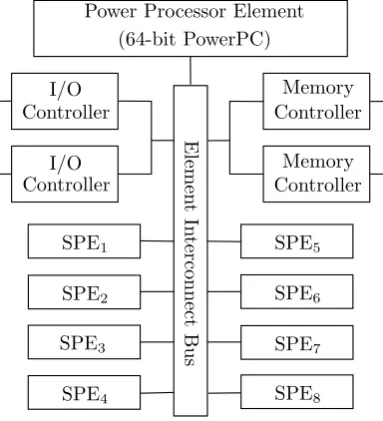
The Vector Floating-Point Unit of the Cell Processor
![Figure 3.2: UltraSparc T2 addition/multiplication datapath [11]](https://thumb-us.123doks.com/thumbv2/123dok_us/1191087.642356/35.595.138.459.234.602/figure-ultrasparc-t-addition-multiplication-datapath.webp)
![Figure 3.3: Intel Itanium architecture [4]](https://thumb-us.123doks.com/thumbv2/123dok_us/1191087.642356/38.595.69.525.332.638/figure-intel-itanium-architecture.webp)
![Figure 3.6: Dual path floating-point adder [21]](https://thumb-us.123doks.com/thumbv2/123dok_us/1191087.642356/44.595.116.485.95.349/figure-dual-path-oating-point-adder.webp)
![Figure 3.7: Reconfigurable floating-point integer adder [24]](https://thumb-us.123doks.com/thumbv2/123dok_us/1191087.642356/46.595.112.481.254.558/figure-recongurable-oating-point-integer-adder.webp)