The in uence of a target motion model on the exact Bayesian filter recursion; research by particle filtering

(1)

The influence of a target motion model on the exact Bayesian

filter recursion; research by particle filtering

Master thesis - Applied Mathematics - August 2010

J.J. van der Valk

(2)

(3)

Written by Aniek van der Valk Master Thesis

August 2010

The influence of a target motion model on the exact Bayesian filter recursion; research by particle filtering

Supervisors:

Prof. Dr. Anton A. Stoorvogel (University of Twente, the Netherlands) Dr. ir. Henk A. P. Blom (National Aerospace Laboratory NLR, the Netherlands)

University of Twente Department of Applied Mathematics Mathematical System and Control Theory P.O. Box 217 7500 AE Enschede The Netherlands

(4)

(5)

Preface

This is my thesis for the Master ’Applied Mathematics’ at University of Twente, carried out at National Aerospace Laboratory NLR. The aim of my thesis is to investigate the influence of a target motion model on the exact Bayesian filter equations. Particle filtering will be used as tool to get more insight in the Bayesian filter recursion.

NLR is a Dutch organization that identifies, develops and applies high-tech knowledge in the aviation and aerospace sectors. At NLR I performed my research at the Air Transport Safety Institute (ATSI). NLR-ATSI is a consultancy and research organization that develops and applies world-class knowledge and expertise to improve air transport safety. NLR-ATSI supports worldwide stakeholders in air transport to understand and resolve complex safety implications of the new technologies and operations necessary to accommodate growth in air transport. Amongst customers of the safety institute are air navigation service providers, aviation authorities, airports and airlines.

I would like to thank my supervisors Dr. ir. Henk A. P. Blom at NLR and Prof. dr. Anton A. Stoorvogel at University of Twente for their supervision and support during my research. Henk, I enjoyed working with you very much and I appreciate a lot that you always found time to answer my questions. Anton, during our meetings you have given me a lot of new insights by approaching from another perspective. I would also like to thank Dr. Jaroslav Krystul for his willingness to be in the graduation committee.

I am very grateful to NLR for giving me the opportunity to perform my research. I would like to thank the members of ATSI for their interesting conversations during the lunch colloquia. Special thanks to Dr. ir. Mariken Everdij for her help with LateX and to ir. Edwin Bloem for his help with Matlab. Thanks to the members of NLR-ATTS for their interesting con-versations during lunch, and also for letting me assist them with their experiments on NLR simulators as an F16 pilot, helicopter pilot or UAV operator. Many thanks to my colleagues Stefan, Waldo, Fedde, Frank, Anneloes, Veronica and Andrew for the great time we had, for the good talks and the fun with ping pong or rugby. Above all, I would like to thank Kelvin and my family and friends for their support and inspiration.

(6)

(7)

Summary

The goal of this thesis is to find out what role the underlying target motion model plays in tracking problems with S-turns. The target motion model is a hybrid stochastic dynamic model taking into account the state of the object and its mode. Furthermore, the observation process also satisfies a hybrid stochastic dynamic model.

To achieve this goal we derive the exact Bayesian filter recursion for several motion models and observation processes. We use Particle filtering to evaluate the Bayesian filter equations numerically.

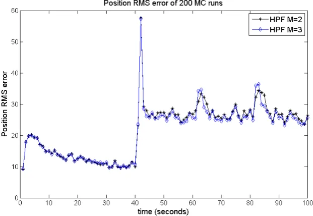
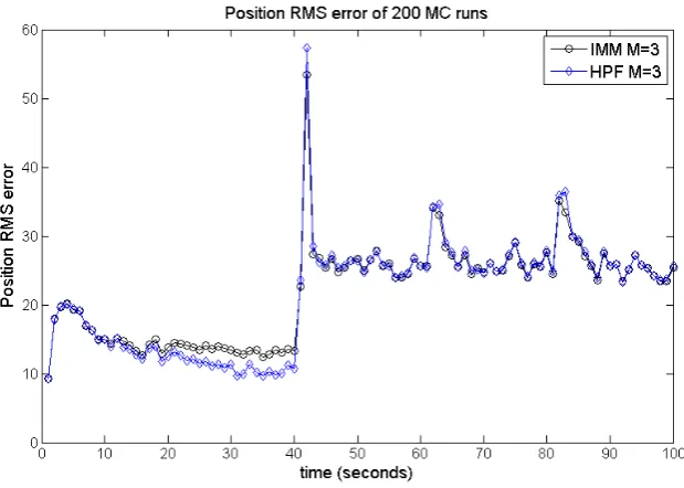
In this thesis results are given of Monte Carlo simulations for the Hybrid Particle filter and the IMM filter algorithm for several different target motion models. Results show that all filters perform relatively well, when the target is switching between acceleration and deceleration. The results show no effect of the tracking problems caused byS-turns we expected.

For all tested filter scenarios IMM performs better than HPF. In most of the filter scenarios, IMM and HPF using the target motion model with three modes perform better than IMM and HPF using the target motion model with two modes.

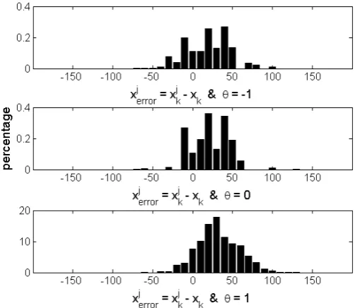
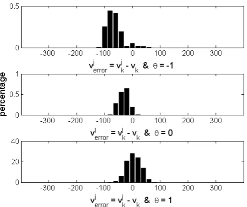
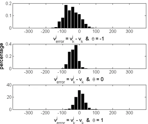
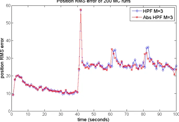
Furthermore, results of two models with three modes show that the choice for a target motion model does effect the performance of HPF. We used a target motion model that permits the target to have a positive acceleration in deceleration mode because the prior deceleration value is assumed to satisfy a Gaussian distribution. The HPF filter using this model performs worse than the HPF filter using a model that does not permit the target to have a positive acceleration in deceleration mode.

(8)

(9)

List of abbreviations

Abs HPF HPF using the model with non-Gaussian acceleration noise from section 8.4 ARTAS ATC Radar Tracker and Server

ATC air traffic control

ATSI Air Transport Safety Institute

CKB Chapman-Kolmogorov-Bayes

HPF Hybrid Particle Filter

i.i.d. independent and identically distributed IMM Interacting Multiple Model

IS importance sampling

MC Monte Carlo

NLR National Aerospace Laboratory NLR

PF Particle Filter

SIR Sampling Importance Resampling UAV Unmanned Aerial Vehicle

List of symbols

a measurable function

abs absolute value

A1 measurable function

A2 measurable function

B1 measurable function

B2 measurable function

ct constant with respect to (x, η)

C1 measurable function

C2 measurable function

χ 0−1 indicator

δ Dirac delta-function

exp Exponential function

η ∈_M parameter

F ∈_Rn×n _constant

fY(y) probability density function of Y =y

fX,Y(x, y) joint probability density function of (X, Y) = (x, y)

f_X|Y(x|y) conditional probability density of X=x given Y =y

g measurable function

G∈_Rm×m0 _{measurable function}

h measurable function

H ∈Rn×m measurable function

i∈_N parameter

I(fk) expectation of fk

(10)

j ∈_N parameter

k∈N parameter

K ∈_R constant

Kk measurable function

L∈Rn×n constant

m dimension ofyk

m0 dimension of the measurement noise

M ∈N constant

M set of M discrete modes

µ∈_Rn _{mean of the process} _{_x

k =x|Yk}

µθ,j₀ initial weight of particle j in mode θ

n dimension ofxk

n0 dimension of the acceleration noise

Np number of particles

Nef f effective sample size

Nthres threshold sample size

N_E,V Gaussian distribution on Rn with parametersE and V

ν_iθ,j i.i.d. standard Gaussian variables of dimension one, independent of θ, j pxk(x) probability density function of xk=x

pXk(X) probability density function of Xk=X pxk|Yk(xk) conditional density of xk =x givenYk p_x_k+1_,x_k|Yk(x, x

0₎ _{joint conditional probability density function of (}_x

k+1, xk) = (x, x0) givenYk

p_y_k+1|xk+1(yk+1|x) conditional likelihood of the realizationyk+1 ∈R

m _{of the process} _{_y k}

at moment k+ 1 given xk+1 =x∈Rn

pk measurable function

pθ₀ initial mode probability of mode θ p{X=x} probability thatX =x

πθη probability that the process {θk} at momentk+ 1 equalsη, i.e. θk+1=η,

given that at moment kthe process{θk} equalsθ, i.e. θk=θ

Π transition probability matrix with componentsπθη

q ∈_R constant

Q∈Rn×n covariance matrix of the process {wk}

Qk measurable function

r ∈_Rn _constant

r1∈R constant

r2∈R constant

rn amount of simulation runs

Rk measurable function

R set of real numbers

S ∈_Rn×n _constant

σa standard deviation of the acceleration noise

σm standard deviation of the measurement error

Σ∈_Rn×n _{variance of the process}_{_x

k=x|Yk}

T ∈N constant

θ∈_M parameter

(11)

{vk} sequence of i.i.d. standard Gaussian variables of dimensionm,

independent of{wk}

{wk} zero mean Gaussian white noise process with covarianceQ

x∈_Rn _parameter

x0 ∈Rn parameter

X ∈_Rn _{random vector}

x0 exact initial state

xθ,j₀ initial state of particlej in modeθ

{xk} Euclidean valued stochastic process

ˆ

xk,i filter estimation ofxk in runiat momentk

ˆ

xHP F

k output of the HPF cycle

Xk={xs;s≤k} the realization of the process{xk} up to and including momentk

{yk} observation process which observes the statexk

Y ∈_Rn _{random vector}

Yk={ys;s≤k} the realization of the process{yk}up to and including moment k

zk measurable function

(12)

(13)

1 Introduction

In air traffic control (ATC), ARTAS (ATC Radar Tracker and Server) forms a critical link between the radars and the air traffic controller. ARTAS is a system designed to establish an accurate air situation picture of all traffic over a well-defined geographical area (e.g. the Euro-pean Civil Aviation Conference), and to distribute the relevant surveillance information to a community of user systems. Amongst other techniques, ARTAS makes use of the Interacting Multiple Model (IMM) filter algorithm and a heuristic such that S-turns of objects are well processed. The question is; is this heuristic necessary because the IMM is an approximation or is this heuristic necessary because the underlying model causes a problem?

The goal of this research is to find out what role the underlying model plays in tracking prob-lems withS-turns. The type of underlying model considered is as follows. For an aircraft a motion model is assumed. This motion model is a hybrid stochastic dynamic model taking into account the state (x-coordinate, y-coordinate, velocity, etc.) of the aircraft and its mode (turn left, straight ahead or turn right). Furthermore, the observation process also satisfies a hybrid stochastic dynamic model.

Rather than continuing with an approximate filter, in this study we use an exact Bayesian filter for the motion model and the observation process. Then we will use particle filtering to evaluate the Bayesian filter equations numerically. If we then find the same phenomenon, we know that the nature of the problem lies in the motion model and observation process.

Thus, this thesis is about the influence of the motion model on the exact Bayesian filter equations. The research question is: ’How does the choice for a certain motion model affect the exact Bayesian filter equations?’

The outline of this thesis will be as follows. First we will derive exact Bayesian filter recur-sions for several models. Section 2 presents an exact filter recursion for an Euclidean valued state model. In section 3 the exact Bayesian filer recursion for a hidden Markov model is derived. In section 4 we derive the exact Bayesian filter recursion for a hidden Markov model with observer.

(16)

(17)

2 Exact filter recursion for Euclidean state model

Consider the Euclidean valued stochastic process {xk}. The system considered satisfies a

stochastic dynamical model of the form:

xk+1 =F xk+wk (1)

with {wk} is a zero mean, Gaussian white noise process with covariance Q. Furthermore,

xk∈Rn,wk∈Rn

0

and constant F ∈_Rn×n_.

Consider the process{yk} which observes the statexk. {yk} satisfies the following equation:

yk=h(xk) +g(xk)vk (2)

where{vk}is a sequence of i.i.d. (independent and identically distributed) standard Gaussian

variables and independent of wk. Further, yk ∈Rm,vk ∈ Rm

0

, and h and g are measurable mappings ofRn intoRm.

The filtering problem is to estimate the conditional density pxk|Yk(x), x ∈ R

n_{, of} _x

k given

Yk = {ys;s ≤ k}, i.e. Yk denotes the realization of the process {yk} up to and including

momentk. Following [Blom & Bar-Shalom, 2009], we develop the exact recursive equations for

pxk|Yk(x). The characterization of this conditional density consists of two steps. In those two

steps, we make use of Bayes’ rule [Bagchi, 1993]. Bayes’ rule states that for two random vectors

X = [X1, ..., Xn]T and Y = [Y1, ..., Yn]T, with joint probability density function fX,Y(x, y)

andfY(y)6= 0, the conditional probability density of X given Y is defined by

f_X|Y(x|y) =

fX,Y(x, y)

fY(y)

(3)

The first step is a Chapman-Kolmogorov equation [Bagchi, 1993] for the evolution ofxkfromk

tok+1, i.e. the characterization ofpxk+1|Yk(x) as a function ofpxk|Yk(x). Letpxk+1,xk|Yk(x, x

0₎

denote the conditional density ofxk+1 =x and xk=x0 given the realizationYk:

p_x_k+1|Yk(x) =

Z

x0_∈ Rn

p_x_k+1_,x_k|Yk(x, x

0₎_dx0

= Z

x0_∈ Rn

pxk+1|xk,Yk(x|x

0₎_p

xk|Yk(x

0₎_dx0

= Z

x0_∈ Rn

pxk+1|xk(x|x

0

)pxk|Yk(x

0

)dx0 (4)

Note that equation (4) uses the transition densitypxk+1|xk(x|x

0_{). This transition density can}

be expressed as follows. Since xk =x0 is given, the expression F x0 is deterministic. Now wk

is zero mean Gaussian white noise with covarianceQ, thusxk+1 given xk=x0 is a Gaussian

(18)

distribution forxk+1 given xk=x0:

p_x_k+1|xk(x|x

0_{) =} exp

−1

2[x−F x

0_]T_Q−1_[_x₋_{F x}0_]

Det{2πQ}1/2 (5)

Substituting this in (4) yields:

p_x_k+1|Yk(x) =

Z

x0_∈ Rn

exp−1

2[x−F x

0_]T_Q−1_[_x₋_{F x}0_]

Det{2πQ}1/2 pxk|Yk(x

0₎_dx0 ₍₆₎

The second step is the Bayes measurement update, i.e. the characterization ofpxk+1|Yk+1(x)

as a function of pxk+1|Yk(x). In the evaluation of this step, we use Bayes’ rule.

pxk+1|Yk+1(x) =

pxk+1,yk+1|Yk(x, yk+1) pyk+1|Yk(yk+1)

= pyk+1|xk+1,Yk(yk+1|x)pxk+1|Yk(x)

pyk+1|Yk(yk+1)

= pyk+1|xk+1(yk+1|x)pxk+1|Yk(x) p_y_k+1|Yk(yk+1)

(7)

Now {vk} in (2) is a sequence of i.i.d. standard Gaussian variables. Thus the mean of vk

equals zero and the variance ofvk equals them0×m0 identity matrix. For givenxk =x, the

expression h(xk) in (2) is deterministic. This means that{yk|xk =x} is a Gaussian process

with mean h(x) and variance g(x)g(x)T. This leads to the following multivariate normal distribution foryk given xk=x:

pyk|xk(y|x) =

exp−1₂[y−h(x)]T[g(x)g(x)T]−1[y−h(x)]

Det{2πg(x)g(x)T_}1/2 (8)

The conditional likelihoodpyk+1|xk+1(yk+1, x) of the realizationyk+1 ∈R

m _{of the process}_{_y k}

at momentk+ 1 given xk+1 =x, is in this case a function ofx;

p_y_k+1|xk+1(yk+1|x) =

exp −1

2[yk+1−h(x)]

T_[_g₍_x₎_g₍_x₎T_]−1_[_y

k+1−h(x)]

Det{2πg(x)g(x)T_}1/2 (9)

Further the conditional likelihoodp_y_k+1|Yk(yk+1) of the realization yk+1 ∈R

m _{of the process}

{yk} at moment k+ 1 given Yk ={ys;s≤k}, is x-invariant. This constant with respect to

x can be found for example through normalization of the conditional density pxk|Yk(x). We

denote the conditional likelihoodp_y_k+1|Yk(yk+1) byct, because the likelihood could depend on

other variables e.g. time. Thus,

pyk+1|Yk(yk+1) =ct (10)

Now substituting (9) into (7) yields:

pxk+1|Yk+1(x) =

exp−1

2[yk+1−h(x)]

T_[_g₍_x₎_g₍_x₎T_]−1_[_y

k+1−h(x)] ctDet{2πg(x)g(x)T}1/2

(19)

Substituting (6) into (11) yields:

pxk+1|Yk+1(x)

= exp

−1

2[yk+1−h(x)]

T_[_g₍_x₎_g₍_x₎T_]−1_[_y

k+1−h(x)]

ctDet{2πg(x)g(x)T}1/2

· Z

x0_∈ Rn

exp

−1₂[x−F x0]T_Q−1_[_x₋_{F x}0_]

Det{2πQ}1/2 pxk|Yk(x

0

)dx0 (12)

This is a recursive equation for p_x_k|Yk(x).

Note that if h(x) = Hx and g(x) = G, the system is linear and we can use the Kalman filter to estimate the state xk from the observations Yk = {ys;s ≤ k} [Bagchi, 1993]. We

choose to use the recursive equation for the conditional densityp_x_k|Yk(x), because we want to

investigate the exact filter equations.

2.1 Further evaluation

In general analytical reduction of (12) is not feasible. An exceptional case however is when

h(x) =Hxand g(x) =Gand the conditional density p_x_k|Yk(x) is Gaussian with mean µand

variance Σ. In that case we can further evaluate recursive equation (12);

p_x_k+1|Yk+1(x)

= exp

−1₂[yk+1−Hx]T[GGT]−1[yk+1−Hx]

ctDet{2πGGT}1/2

· Z

x0_∈ Rn

exp−1₂[x−F x0]TQ−1[x−F x0] Det{2πQ}1/2

exp−1₂(x0−µ)TΣ−1(x0−µ) Det{2πΣ}1/2 dx

0

(13)

The integral in equation (13) can be written as:

Z

x0_∈ Rn

exp −1

2[x−F x

0_]T_Q−1_[_x₋_{F x}0_]

Det{2πQ}1/2

exp −1

2(x

0₋_µ₎T_Σ−1₍_x0₋_µ₎

Det{2πΣ}1/2 dx

0

= Z

x0_∈ Rn

exp

−1 2[x

0₋_p_]T_S_[_x0₋_p_]

_exp

−1 2q

Det{2πQ}1/2Det{2πΣ}1/2dx

0 ₍₁₄₎

with

S = FTQ−1F+ Σ−1 (15)

p = S−1(FTQ−1x+ Σ−1µ) (16)

(20)

Note that the inverse ofS does exist because S is positive definite since FTQ−1F ≥0 and Σ−1 >0. Now equation (14) yields:

Z

x0_∈ Rn

exp

−1 2[x

0₋

p]TS[x0−p]

exp−1₂q

Det{2πQ}1/2Det{2πΣ}1/2dx

0

= exp

−1₂q

Det{2πQ}1/2Det{2πΣ}1/2 ·Det

2πS−1 1/2 (18)

and equation (13) yields:

p_x_k+1|Yk+1(x)

= exp

−1₂[yk+1−Hx]T[GGT]−1[yk+1−Hx]

ctDet{2πGGT}1/2

exp−1₂q Det2πS−1 1/2

Det{2πQ}1/2Det{2πΣ}1/2

= K·exp

−1 2[x−r]

T_L_[_x₋_r_]

(19)

with

S = FTQ−1F+ Σ−1

L = Q−1−Q−1F S−1FTQ−1+HT(GGT)−1H (20)

r = L−1[Q−1F S−1Σ−1µ+HT(GGT)−1yk+1] (21)

K = exp

−1 2

µTΣ−1µ−µTΣ−1S−1Σ−1µ+y_kT₊₁(GGT)−1yk+1−rTLr Det

2πS−1 1/2

ct Det{2πGGT}1/2Det{2πQ}1/2Det{2πΣ}1/2

(22)

Note that the inverse ofLdoes exist becauseLis positive definite sinceQ−1>0,Q−1F S−1FTQ−1 ≥ 0 andHT(GGT)−1H ≥0. We can rewrite Las (see Appendix A.1):

L = [FΣFT +Q]−1+HT(GGT)−1H (23)

Because (see Appendix A.2):

Q−1F S−1Σ−1µ = [FΣFT +Q]−1F µ (24)

We can rewriter as:

r = L−1[Q−1F S−1Σ−1µ+HT(GGT)−1yk+1]

= [FΣFT +Q]−1+HT(GGT)−1H−1

[FΣFT +Q]−1F µ+HT(GGT)−1yk+1

(25)

Becausepxk+1|Yk+1(x) is a density, the integral over this density should equal 1. Thus K can

also be found by normalizing the density. That is K should be equal to Det{2πL−1}−1/2_.

And ct can be found in two ways, by using K or by evaluatingpyk+1|Yk(yk+1). If we look at

(21)

variance Σ and the measurementyk+1.

From equation (19) we see that pxk+1|Yk+1(x) is a Gaussian distribution with mean r and

(22)

(23)

3 Exact Bayesian filter recursion for a hidden Markov model

Consider a two-component Markov process{xk, θk}, with{xk}an Euclidean valued stochastic

process and{θk}a discrete valued process. The system considered satisfies a hybrid stochastic

dynamical model of the form:

xk+1 =a(θk+1, xk) +b(θk+1)wk (26)

where wk is a zero mean, Gaussian white noise process with covariance Q. Further, {θk}

is an M-valued Markov chain with transition probability matrix Π with components πθη =

p{θk+1=η|θk=θ}.

The filtering problem is to estimate the conditional densitypθk|Xk(θ) withθ∈M of θk given Xk = {xs;s ≤ k}, i.e. the realization of the process {xk} up to and including moment k.

Following [Blom & Bar-Shalom, 2009], we develop the exact recursive equations forp_θ_k|Xk(θ).

The characterization of this conditional density consists of two steps.

The first step is to characterize the Chapman-Kolmogorov equation for the evolution of xk

fromk tok+ 1, i.e. the characterization of p_θ_k+1|Xk(θ) as a function of pθk|Xk(θ):

pθk+1|Xk(η) =

X

θ∈_M

pθk+1,θk|Xk(η, θ) =

X

θ∈_M

pθk+1|θk,Xk(η|θ)pθk|Xk(θ) =

X

θ∈_M

πθηpθk|Xk(θ) (27)

The second step is the Bayes measurement update, i.e. the characterization ofp_θ_k+1|Xk+1(θ)

as a function of pθk+1|Xk(θ). Using Bayes’ rule we have

pθk+1|Xk+1(η) =

pθk+1,xk+1|Xk(η, xk+1) p_x_k+1|Xk(xk+1)

= pxk+1|θk+1,Xk(xk+1|η)pθk+1|Xk(η)

pxk+1|Xk(xk+1)

= pxk+1|θk+1,xk(xk+1|η, xk)pθk+1|Xk(η)

pxk+1|Xk(xk+1)

(28)

Note that equation (28) uses the conditional density pxk+1|θk+1,xk(x|η, x

0_{). Given the pair}

(θk+1 = η, xk = x0) the expression a(η, x0) is deterministic and wk is a zero mean Gaussian

white noise process with covariance Q. Therefore, the process {xk+1|θk+1 =η, xk=x0} is a

Gaussian process with meana(η, x0) and covarianceb(η)Qb(η)T. Now the conditional density

pxk+1|θk+1,xk(x|η, x

0_{) can be expressed as follows:}

0_{) =} exp

−1₂[x−a(η, x0)]T(b(η)Qb(η)T)−1[x−a(η, x0)]

(24)

The conditional likelihood p_x_k+1|θk+1,xk(xk+1|η, xk) of the realization of xk+1 ∈ R

n _{of the}

process {xk} at moment k+ 1, given the realization of xk ∈ Rn of the process {xk} at

momentk, and θk+1 =η, is in this case a function ofη:

p_x_k+1|θk+1,xk(xk+1|η, xk) =

exp −1

2[xk+1−a(η, xk)]

T₍_b₍_η₎_Qb₍_η₎T₎−1_[_x

k+1−a(η, xk)]

Det{2πb(η)Qb(η)T_}1/2 (30)

Further, the conditional likelihood p_x_k+1|Xk(xk+1) of the realizationxk+1∈R

n_{of the process}

{xk} at moment k+ 1, given Xk = {xs;s ≤ k}, is (x, η)-invariant. This constant with

respect to (x, η) can be found for example through normalization of the conditional density

p_θ_k|Xk(θ). We denote the conditional likelihood pxk+1|Xk(xk+1) byct, because the likelihood

could depend on other variables e.g. time. Thus,

p_x_k+1|Xk(xk+1) =ct (31)

Now substituting (30) and (31) into (28) yields:

p_θ_k+1|Xk+1(η) =

exp −1

2[xk+1−a(η, xk)]

T₍_b₍_η₎_Qb₍_η₎T₎−1_[_x

k+1−a(η, xk)]

ct Det{2πb(η)Qb(η)T}1/2

p_θ_k+1|Xk(η)

(32) Substituting (27) into (32) yields:

pθk+1|Xk+1(η) =

exp−1₂[xk+1−a(η, xk)]T(b(η)Qb(η)T)−1[xk+1−a(η, xk)]

ct Det{2πb(η)Qb(η)T}1/2

X

θ∈_M

πθηpθk|Xk(θ)

(33)

(25)

4 Exact Bayesian filter recursion for a hidden Markov model

with observer

Consider a two-component Markov process{xk, θk}with{xk}an Euclidean valued stochastic

process and{θk}a discrete valued process. The system considered satisfies a hybrid stochastic

dynamical model of the form:

xk+1 =a(θk+1, xk) +b(θk+1)wk (34)

where wk is a zero mean, Gaussian white noise process with covariance Q. Further, {θk}

is an M-valued Markov chain with transition probability matrix Π with components πθη =

p{θk+1=η|θk=θ}.

Consider the process{yk} which observes the statexk. {yk} satisfies the following equation:

yk =h(θk, xk) +g(θk, xk)vk (35)

where{vk}is a sequence of i.i.d. standard Gaussian variables of dimension m0 and

indepen-dent ofwk.

The filtering problem is to estimate the joint conditional densitypxk,θk|Yk(x, θ),x∈R

n_,_θ_∈

M,

of the pair (xk, θk) given Yk={ys;s≤k}, i.e. the realization of the process {yk}up to and

including moment k. Following [Blom & Bar-Shalom, 2009], we develop the exact recursive equations for pxk,θk|Yk(x, θ). The characterization of this conditional density consists of two

steps.

The first step is to characterize the Chapman-Kolmogorov equation for the evolution of the pair (xk, θk) from k to k+ 1, i.e. the characterization of pxk+1,θk+1|Yk(x, θ) as a function of p_x_k_,θ_k|Yk(θ):

pxk+1,θk+1|Yk(x, η) =

Z

x0_∈ Rn

pxk+1,xk,θk+1|Yk(x, x

0

, η)dx0

= Z

x0_∈ Rn

pxk+1,θk+1|xk,Yk(x, η|x

0

)pxk|Yk(x

0

)dx0

= Z

x0_∈ Rn

X

θ∈M

p_x_k+1_,θ_k+1_,θ_k|xk,Yk(x, η, θ|x

0₎_p

xk|Yk(x

0₎_dx0

= Z

x0_∈ Rn

X

θ∈M

p_x_k+1_,θ_k+1|xk,θk,Yk(x, η|x

0_{, θ}₎_p

θk|Yk(θ)pxk|Yk(x

0₎_dx0

= Z

x0_∈ Rn

X

θ∈_M

pxk+1,θk+1|xk,θk(x, η|x

0_{, θ}₎_p

xk,θk|Yk(x

(26)

Note that equation (36) uses the transition densityp_x_k+1_,θ_k+1|xk,θk(x, η|x

0_{, θ}_{). This transition}

density can be expressed as follows:

p_x_k+1_,θ_k+1|xk,θk(x, η|x

0_{, θ}₎ ₌ _p

xk+1|θk+1,xk,θk(x|η, x

0_{, θ}₎_p

θk+1|xk,θk(η|x

0_{, θ}₎

= pxk+1|θk+1,xk(x|η, x

0₎_p

θk+1|θk(η|θ)

= pxk+1|θk+1,xk(x|η, x

0

)πθ,η (37)

For a given (θk+1 =η, xk=x0), the expression a(η, x0) is deterministic. Nowwk is zero mean

Gaussian white noise with covarianceQ. Thus{xk+1|θk+1 =η, xk =x0}is a Gaussian process

with meana(η, x0) and covarianceb(η)Qb(η)T_{. This leads to the following multivariate normal}

distribution for xk+1 given (θk+1 =η, xk =x0):

0

) = exp

−1₂[x−a(η, x0)]T(b(η)Qb(η)T)−1[x−a(η, x0)]

Det{2πb(η)Qb(η)T_}1/2 (38)

This leads to the following expression for pxk+1,θk+1|xk,θk(x, η|x

0_{, θ}_):

0_{, θ}₎ ₌ _p

xk+1|θk+1,xk(x|η, x

0₎_p

θk+1|θk(η|θ)

= exp

−1

2[x−a(η, x

0_)]T₍_b₍_η₎_Qb₍_η₎T₎−1_[_x₋_a₍_{η, x}0_)]

Det{2πb(η)Qb(η)T_}1/2 πθη

(39)

Substituting this into (36) yields:

p_x_k+1_,θ_k+1|Yk(x, η)

= Z

x0_∈ Rn

X

θ∈_M

exp−1₂[x−a(η, x0)]T(b(η)Qb(η)T)−1[x−a(η, x0)]

Det(2πb(η)Qb(η)T₎1/2 πθη pxk,θk|Yk(x

0

, θ)dx0

= Z

x0_∈ Rn

exp −1

2[x−a(η, x

0_)]T₍_b₍_η₎_Qb₍_η₎T₎−1_[_x₋_a₍_{η, x}0_)]

Det(2πb(η)Qb(η)T₎1/2

X

θ∈M

πθη pxk,θk|Yk(x

0_{, θ}₎_dx0

(40)

The second step is the Bayes measurement update, i.e. the characterization ofp_x_k+1_,θ_k+1|Yk+1(x, θ)

as a function ofpxk+1,θk+1|Yk. Using Bayes’ rule we have

p_x_k+1_,θ_k+1|Yk+1(x, η) =

p_y_k+1|xk+1,θk+1(yk+1|x, η)pxk+1,θk+1|Yk(x, η) p_y_k+1|Yk(yk+1)

(41)

Now {vk} in (83) is a sequence of i.i.d. standard Gaussian variables. Thus the mean of vk

equals zero and the variance ofvkequals them0×m0identity matrix. For a given pair (xk, θk),

the expressionh(θk, xk) in (83) is known. This means that {yk+1|xk+1 = x, θk+1 = η} is a

Gaussian process with mean h(η, x) and varianceg(η, x)g(η, x)T. This leads to the following multivariate normal distribution foryk+1 given the pair (xk+1=x, θk+1=η):

pyk+1|xk+1,θk+1(y|x, η) =

exp−1

2[y−h(η, x)]

T₍_g₍_{η, x}₎_g₍_{η, x}₎T₎−1_[_y₋_h₍_{η, x}_)]

(27)

p_y_k+1|xk+1,θk+1(yk+1|x, η) is the conditional likelihood of the realization of yk+1 ∈ R

m _{of the}

process {yk} at moment k+ 1, given xk+1 = x and θk+1 = η. The conditional likelihood pyk+1|xk+1,θk+1(yk+1|x, η) is in this case a function of xand η:

pyk+1|xk+1,θk+1(yk+1|x, η) =

exp−1₂[yk+1−h(η, x)]T(g(η, x)g(η, x)T)−1[yk+1−h(η, x)]

Det{2πg(x, η)g(x, η)T_}1/2

(43)

Further, the conditional likelihoodpyk+1|Yk(yk+1) of the realizationyk+1 ∈R

m _{of the process}

{yk}at momentk+ 1, givenYk={ys;s≤k}, is a (x, η)-invariant. This constant with respect

to (x, η) can be found for example through normalization of the conditional densitypxk,θk|Yk.

We denote the conditional likelihoodpyk+1|Yk(yk+1) byct, because the likelihood could depend

on other variables e.g. time. Thus,

pyk+1|Yk(yk+1) =ct (44)

Now substituting (43) into (41) yields:

pxk+1,θk+1|Yk+1(x, η)

= exp

−1

2[yk+1−h(η, x)]

T₍_g₍_{η, x}₎_g₍_{η, x}₎T₎−1_[_y

k+1−h(η, x)] ct Det{2πg(x, η)g(x, η)T}1/2

p_x_k+1_,θ_k+1|Yk(x, η)

(45)

Substituting (40) into (45) yields:

p_x_k+1_,θ_k+1|Yk+1(x, η)

= exp

−1₂[yk+1−h(η, x)]T(g(η, x)g(η, x)T)−1[yk+1−h(η, x)]

ct Det{2πg(x, η)g(x, η)T}1/2

· Z

x0_∈ Rn

exp−1₂[x−a(η, x0)]T(b(η)Qb(η)T)−1[x−a(η, x0)] Det{2πb(η)Qb(η)T_}1/2

X

θ∈_M

πθη pxk,θk|Yk(x

0

, θ)dx0

(46)

This is a recursive equation forpxk+1,θk+1|Yk+1(x, η). We can rewrite this equation as follows

(see Appendix A.3):

p_x_k+1_,θ_k+1|Yk+1(x, η)

= Z

x0_∈ Rn

exp−1₂(r1+r2)

ct(Det{2πg(x, η)g(x, η)T}Det{2πb(η)Qb(η)T})1/2

X

θ∈_M

πθη pxk,θk|Yk(x

0_{, θ}₎_dx0

(47)

where

(28)

(29)

5 Particle filter

5.1 Introduction

To investigate the influence of a target motion model on the exact Bayesian filter equations, we may simulate this filtering process with a particle filter. Since their introduction in 1993 [Gordon et al., 1993], particle filters have become a very popular class of numerical methods for the solution of optimal estimation problems in non-linear non-Gaussian scenarios. In 1993 the particle filter was known as the bootstrap filter. Particle methods are a subset of the class of methods known as Sequential Monte Carlo methods. In comparison with the stan-dard approximation methods, such as the Extended Kalman Filter, the principal advantage of particle methods is that they do not rely on any local liberalization technique or any func-tional approximation.

According to the strong law of large numbers, the approximation density almost sure converges to the exact conditional density if the number of particles used in the approximation is going to infinity [van der Merwe et al., 2000]. This is why a particle filter has been selected to investigate the influence of a target motion model on the exact conditional density. As many particles as necessary for a good enough approximation of the joint conditional density will be used. The purpose is not to decrease the number of particles but to investigate the joint conditional density with a particle filter as an arbitrary accurate numerical approximation technique.

5.2 The filtering problem

Following [Blom & Bloem, 2007], let {xk, θk} be a hybrid state process, with xk assuming

values inRnandθkassuming values in a finite setMof possible modes, be a hidden state

pro-cess to be estimated from noisy observations{yk}, with yk assuming values in Rm. Consider

the following system of stochastic difference equations, on [0, T],T <∞,

xk = a(θk, xk−1, wk) (50)

θk = c(θk−1, xk−1, uk) (51)

yk = h(θk, xk, vk) (52)

where the pair (xk, θk) represents the hybrid system state, andykrepresents the observation at

momentk,{wk}and {vk}are independent sequences of i.i.d. standard Gaussian variables of

dimensionn0 andm0 respectively,{uk}is an{wk, vk}-independent sequence of i.i.d. standard

uniform random variables,{wk, vk, uk}is independent of theRn×Mvalued initial condition

(x0, θ0), with M a set of M discrete modes. Furthermore,a andh are measurable mappings

of M×Rn×Rn

0

into Rn and M×Rn×Rm

0

into Rm respectively, and c is a measurable

mapping ofM×Rn×[0,1] intoM. The mappingsa,candhare time-invariant for notational

simplicity only.

The filtering problem is to estimate the joint conditional density-probability pxk,θk|Yk(x, θ), x∈_Rn_,_θ_∈

(30)

5.3 SIR particle filter

A common particle filter used in nonlinear filtering studies is the Sampling Importance Resam-pling (SIR) particle filter. It has shown to form an elegant and general approach towards the numerical evaluation of the conditional density of the Chapman-Kolmogorov-Bayes (CKB) filter recursion. The SIR particle filter is also capable in approximating the CKB equations of a stochastic hybrid Markov process{xk, θk}, withxk assuming values inRn, andθkassuming

values in a finite setM of possible modes. Therefore the SIR particle filter shall be used.

The SIR particle filter uses Np particles. Each particle j has two-components (xj_k, θj_k) at

momentk, withxj_k assuming an Euclidean value and θj_k assuming a discrete value.

Now we will present the SIR particle filter cycle applied to the model given in section 5.2. Each SIR particle filter cycle fromk−1 to kconsists of three steps [Blom & Bloem, 2007]:

Evolution. For each of theNp particles at moment k−1, draw a new hybrid particle

(¯xj_k,θ¯j_k) according to the Chapman-Kolmogorov transition kernel. That is for each particle sample a state at moment k given the state of that particle at moment k−1, the transition probability matrix Π for theM-valued Markov chain{θk}and the hybrid

stochastic dynamical model for the process {xk}.

Correction. For each of theNp particles evaluate ¯µj_kas the likelihood of the

measure-ment at momeasure-ment k, given (¯xj_k,θ¯j_k) and normalize the resulting ¯µj_k’s. In this way, each particle is given a weight on the basis of the measurement and the sampled state of the particle.

Resampling. Draw Np independently identically distributed (i.i.d.) hybrid particle

values (xj_k, θj_k), from the sum of ¯µ_kj weighted Dirac measures at (¯xj_k,θ¯j_k). That is we draw Np new particles and each particle (¯xj_k,θ¯j_k) is drawn with probability ¯µj_k.

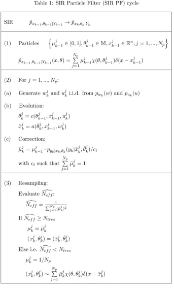
Table 1 gives an overview of the SIR particle filter cycle for the filter problem setting of equations (50)-(52). In this table, χ(θ, θ_kj₋₁) is a 0 −1 indicator with χ(θ, θ_kj₋₁) = 1 if

θ = θ_kj₋₁. Note that p_y_k|xk,θk(yk|¯x

j k,θ¯

j

k) is the likelihood of the measurement at moment k

given (¯xj_k,θ¯j_k). The table without step (3) resampling, i.e. Ntres = 0, is given by [Blom &

(31)

[image:31.595.131.475.109.679.2]

Table 1: SIR Particle Filter (SIR PF) cycle

SIR p˜_x_k₋₁_,θ_k₋₁|Yk−1 →p˜xk,θk|Yk

(1) Particles nµj_k₋₁∈[0,1], θ_kj₋₁ ∈_M, xj_k₋₁ ∈_Rn_;_j_{= 1}_{, ..., N} p

o

˜

p_x_k₋₁_,θ_k₋₁|Yk−1(x, θ) =

Np

P

j=1

µj_k₋₁χ(θ, θj_k₋₁)δ(x−xj_k₋₁)

(2) Forj= 1, ..., Np:

(a) Generatewj_k and uj_k i.i.d. from pwk(w) and puk(u)

(b) Evolution:

¯

θj_k=c(θ_kj₋₁, xj_k₋₁, uj_k)

¯

xj_k =a(¯θj_k, xj_k₋₁, wj_k)

(c) Correction:

¯

µj_k=µj_k₋₁·pyk|xk,θk(yk|¯x

j k,θ¯

j k)/ct

withct such that Np

P

j=1

¯

µj_k= 1

(3) Resampling:

Evaluate N[ef f:

[

Nef f = PNp1

j=1(¯µ j k)2

IfN[ef f ≥Ntres

µj_k= ¯µj_k

(xj_k, θ_kj) = (¯xj_k,θ¯_kj)

Else i.e. N[ef f < Ntres

µj_k= 1/Np

(xj_k, θj_k)∼

Np

P

j=1

¯

(32)

5.4 Convergence of a particle filter

This subsection explains from a theoretical point of view why the SIR particle filter gives a good estimation of the exact Bayesian filter equations.

5.4.1 Problem statement

Following [Doucet, 1998], we estimate recursively in time the distribution pXk,Θk|Yk(X,Θ),

where Xk = {x0, ..., xk}, Θk = {θ0, ..., θk} and Yk = {y0, ..., yk}, and with X ∈ R(k+1)×n,

Θ ∈ _Mk+1_{. Why we use this approach will be shown further on. From} _p

Xk,Θk|Yk(X,Θ) we

obtain p_x_k_,θ_k|Yk(x, θ) by marginalizing over the variables that are not of interest. Thus, for pXk,Θk|Yk(X,Θ) =pXk−1,xk,Θk−1,θk|Yk(X

0_{, x,}_Θ0_{, θ}_):

pxk,θk|Yk(x, θ) =

X

Θ0_∈ Mk

Z

X0_∈ Rk×n

pXk−1,xk,Θk−1,θk|Yk(X

0

, x,Θ0, θ)dX0 (53)

This implies that we can estimate recursively in time the distribution pxk,θk|Yk(x, θ) from

marginalizing the estimation ofp_X_k_,_Θk|Yk(X,Θ).

Further, the filtering problem is also to estimate the expectation

I(fk),Ep_Xk,Θ_k|_Yk(X,Θ)(fk(X,Θ)) =

X

Θ∈Mk+1

Z

X∈_R(k+1)×n

fk(X,Θ)pXk,Θk|Yk(X,Θ)dX (54)

for any p_X_k_,_Θk|Yk(X,Θ)-integrable fk : R

(n+1)×nx _×

Mk+1 → R. In other words, for every

functionfk :R(n+1)×nx×Mk+1 →R for which the integral of fk(X,Θ)pXk,Θk|Yk(X,Θ) with

respect toX exists.

The reason why we use pXk,Θk|Yk(X,Θ) instead of pxk,θk|Yk(x, θ) is because pXk,Θk|Yk(X,Θ)

can be expressed by a recursive formula. In the derivation of this recursive formula, we will use the following:

pA|B(a, b) =

pA,B(a, b)

pB(b)

= pB|A(b|a)pA(a)

pB(b)

(55)

Using this,pXk,Θk|Yk(X,Θ) can be expressed as follows:

p_X_k+1_,_Θk+1|Yk+1(X,Θ) =

p_Y_k+1|Xk+1,Θk+1(Yk+1|X,Θ)pXk+1,Θk+1(X,Θ) pYk+1(Yk+1)

(56)

Due to the stochastic differential equations (50), (51) and (52) of the system,pXk+1,Θk+1(X,Θ)

(33)

pXk+1,Θk+1(X,Θ) = pxk+1,θk+1,Xk,Θk(x, η, X

0_,_Θ0₎

= pxk+1,θk+1|Xk,Θk(x, η|X

0

,Θ0)pXk,Θk(X

0

,Θ0) = pxk+1,θk+1|xk,θk(x, η|x

0

, θ)pXk,Θk(X

0

,Θ0) (57)

Further,pYk+1|Xk+1,Θk+1(Yk+1|X,Θ) can be expressed as:

pYk+1|Xk+1,Θk+1(Yk+1|X,Θ) = pyk+1,Yk|Xk+1,Θk+1(yk+1, Yk|X,Θ)

= pyk+1|Yk,Xk+1,Θk+1(yk+1|Yk, X,Θ)pYk|Xk+1,Θk+1(Yk|X,Θ)

= p_y_k+1|xk+1,θk+1(yk+1|x, η)pYk|Xk,Θk(Yk|X

0_,_Θ0₎ ₍₅₈₎

pYk+1(Yk+1) satisfies:

pYk+1(Yk+1) =pyk+1,Yk(yk+1, Yk) =pyk+1|Yk(yk+1|Yk)pYk(Yk) (59)

Using (56), (57), (58) and (59) we have:

p_X_k+1_,_Θk+1|Yk+1(X,Θ)

= pYk+1|Xk+1,Θk+1(Yk+1|X,Θ)pXk+1,Θk+1(X,Θ)

pYk+1(Yk+1)

= pXk,Θk(X

0_,_Θ0₎_p

Xk,Θk(X

0_,_Θ0₎

pYk(Yk)

0_{, θ}₎_p

xk+1,θk+1|xk,θk(x, η|x

0_{, θ}₎

pyk+1|Yk(yk+1|Yk)

= pXk,Θk|Yk(X

0_,_Θ0₎ pyk+1|xk+1,θk+1(yk+1|x, θ)pxk+1,θk+1|xk,θk(x, η|x

0_{, θ}₎

p_y_k+1|Yk(yk+1|Yk)

(60)

5.4.2 Approximation of a density through particles

Let us assume that we are able to simulateNp i.i.d. random samples{(X_kj,Θj_k);j= 1, ..., Np}

according topXk,Θk|Yk(X,Θ). An approximationpeXk,Θk|Yk(X,Θ) of pXk,Θk|Yk(X,Θ) is given

by:

e

pXk,Θk|Yk(X,Θ) =

1

Np Np

X

j=1

χ(Θ,Θj_k)δ(X−X_kj) (61)

where χ(Θ,Θj_k) is a 0−1 indicator with χ(Θ,Θj_k) = 1 if Θ = Θj_k and with δ(.) the Dirac

(34)

e

INp(fk) =

X

Θ∈Mk+1

Z

X∈_R(k+1)×n

fk(X,Θ)ˆpXk,Θk|Yk(X,Θ)dX=

1

Np Np

X

j=1

fk(Xkj,Θ j

k) (62)

From the strong law of large numbers [Ross, 1996],

P

lim

Np→∞

INp(fk) =I(fk)

= 1 (63)

i.e. INp(fk) converges almost sure toI(fk) whenNp → ∞.

A problem arises when pXk,Θk|Yk(X,Θ) is unknown, because then we cannot sample from p_X_k_,_Θk|Yk(X,Θ). In that case we may use importance sampling (IS). The basic idea of IS

is to choose a so-called importance function πk(X,Θ), which is a probability distribution

from which one can easily sample. Further, the importance functionπk(X,Θ) should satisfy

πk(X,Θ)>0 wheneverpXk,Θk|Yk(X,Θ)>0. Now we can write:

I(fk) =

X

Θ∈_Mk+1

Z

X∈R(k+1)×n

fk(X,Θ)

pXk,Θk|Yk(X,Θ) πk(X,Θ)

πk(X,Θ)dX (64)

= Eπk(X,Θ)[fk(X,Θ)w∗k(X,Θ)] (65)

where

w∗_k(X,Θ) = pXk,Θk|Yk(X,Θ) πk(X,Θ)

(66)

Thus if we simulate Np i.i.d. samples {(Xkj,Θ j

k);j = 1, ..., Np} according to πk(X,Θ), an

approximation ofI(fk) is:

b

I_N∗_p(fk) =

1

Np Np

X

j=1

fk(X_kj,Θj_k)w

∗(j)

k (67)

where the importance weights{w_k∗(j), j = 1, ..., Np}are equal to:

w_k∗(j)=w∗_k(X_k(j),Θ(_kj)) = pXk,Θk|Yk(X (j)

k ,Θ

(j)

k )

πk(X_k(j),Θ(_kj))

= pYk|Xk,Θk(Yk|X (j)

k ,Θ

(j)

k )pXk,Θk(X (j)

k ,Θ

(j)

k )

pYk(Yk)πk(X (j)

k ,Θ

(j)

k )

(68) The estimateIb_N∗

p(fk) is unbiased, i.e. E[Ib

∗

Np(fk)|I(fk)] =I(fk) [Ross, 1996], and converges

almost sure according to the strong law of large numbers towardI(fk) whenNp → ∞[Doucet,

1998].

Note that pYk(Yk) is (X,Θ)-invariant and therefore it can be found by normalization. Let w_k(j) be defined as follows:

w(_kj),pYk(Yk)w

∗(j)

k (69)

(35)

w_k(j) = pYk|Xk,Θk(Yk|X (j)

k ,Θ

(j)

k )pXk,Θk(X (j)

k ,Θ

(j)

k )

πk(X

(j)

k ,Θ

(j)

k )

(70)

Usingw_k(j) rather thanw_k∗(j), then an estimate ofI(fk) becomes:

b

INp(fk) =

1

ck Np

X

j=1

fk(Xkj,Θ j k)w

(j)

k (71)

with

ck =pYk(Yk) (72)

Assumption 1

- n(X_k(j),Θ(_kj));j= 1, ..., Np

o

is a set of i.i.d. vectors distributed according toπk(X,Θ).

- πk(X,Θ)>0 for all (X,Θ)∈(R(k+1)×n,Mk+1) for which pXk,Θk|Yk(X,Θ)>0.

- I(fk) exists and is finite.

For Np finite, Ib_N_p(f_k) is biased, but under assumption 1, asymptotically the strong law of large numbers yields:

P

lim

Np→∞

b

INp(fk) =I(fk)

= 1 (73)

i.e. Ib_N_p(f_k) converges almost sure to I(f_k) when N_p → ∞ [Doucet, 1998].

In order to get the SIR particle filter, we choose the following importance function:

πk(X,Θ) =pXk,Θk(X,Θ) (74)

Note thatpXk,Θk(X,Θ) should satisfy assumption 1.

Now w_k(j) satisfies:

w_k(j)=pYk|Xk,Θk(Yk|X (j)

k ,Θ

(j)

k ) (75)

Using (58), w_k(j₊₁) can be expressed as:

w_k(j₊₁) = pYk+1|Xk+1,Θk+1(Yk+1|X (j)

k+1,Θ (j)

k+1)

= p_Y_k|Xk,Θk(Yk|X (j)

k ,Θ

(j)

k )pyk+1|xk+1,θk+1(yk+1|x (j)

k+1, θ (j)

k+1)

= w_k(j)pyk+1|xk+1,θk+1(yk+1|x (j)

k+1, θ (j)

(36)

5.4.3 Algorithm

The algorithm in table 1 without the resampling step follows from recursive equation (60) in section 5.4.1 and from the approximation of a density through particles in section 5.4.2. We show this in more detail below.

First we sample Np particles according to the importance function π0(x, θ) = px0,θ0(x, θ).

This is step 1 in table 1.

Then we start the SIR particle filter cycle. During the evolution step, we sample (¯x(_kj),θ¯(_kj)) ac-cording to the importance functionπk(xk, θk|Xk−1,Θk−1) =pxk,θk|Xk−1,Θk−1(x, η|X

(j)

k−1,Θ (j)

k−1)

forj= 1, ..., Np, equation (74). These are step 2aand step 2bin table 1.

During the correction step, we evaluate the weights for the particles using equation (76). That

is,w(_kj₊₁) =w(_kj)pyk+1|xk+1,θk+1(yk+1|¯x (j)

k+1,θ¯ (j)

k+1)/cNp with cNp such that

Np

P

j=1

w(_kj₊₁) = 1. This is

step 2c in table 1.

After each cycle, at time k we have the following approximation forpXk,Θk|Yk(X,Θ):

ˆ

pXk,Θk|Yk(X,Θ) =

Np

X

j=1

w_k(j)χ(Θ,Θ_kj)δ(X−X_kj) (77)

The approximation forp_x_k_,θ_k|Yk(x, θ) can be obtained by marginalizing ˆpXk,Θk|Yk(X,Θ) over

the variables that are not of interest. Note that:

ˆ

p_X_k_,_Θk|Yk(X,Θ) = pˆXk−1,xk,Θk−1,θk|Yk(X

0_{, x,}_Θ0_{, θ}₎

=

Np

X

j=1

w(_kj)χ(Θ0,Θj_k₋₁)χ(θ, θ_kj)δ(X0−X_kj₋₁)δ(x−xj_k) (78)

Marginalizing over allXk−1 and Θk−1 yields:

ˆ

pxk,θk|Yk(x, θ) =

X

Θ0_∈ Mk

Z

X0_∈ Rk×n

ˆ

pXk−1,xk,Θk−1,θk|Yk(X

0

, x,Θ0, θ)dX0

= X

Θ0_∈ Mk

Z

X0_∈ Rk×n

Np

X

j=1

w(_kj)χ(Θ0,Θj_k₋₁)χ(θ, θj_k)δ(X0−X_kj₋₁)δ(x−xj_k)dX0

=

Np

X

j=1

w(_kj)χ(θ, θ_kj)δ(x−xj_k) X

Θ0_∈ Mk

χ(Θ0,Θj_k₋₁) Z

X0_∈ Rk×n

δ(X0−X_kj₋₁)dX0

=

Np

X

j=1

(37)

5.4.4 Resampling

The basic idea of resampling methods consists of eliminating the trajectories which have weak normalized importance weights and to multiply trajectories with strong importance weights [Doucet, 1998]. Without resampling, at some point some particles will have very small weights while others will have very large weights. Those particles with large weight will have a big influence. This leads to degeneracy of the algorithm. We adopt as a measure of degeneracy of the algorithm the effective sample sizeNef f. When the estimation of the effective sample

sizeN[ef f is below a fixed thresholdNthres, we use a resampling procedure. The most popular

resampling scheme is the SIR algorithm. This scheme is based on two steps: a first step is an IS step, the second step is a sampling step based on the obtained discrete distribution. That is if N[ef f < Nthres then, for j = 1, ..., Np sample an index i(j) distributed according to the

discrete distribution with Np elements satisfying P{i(j) = l} = w_k(l) for l = 1, ..., Np. Thus

we sample Np values from a discrete distribution that approximates the exact distribution

pXk,Θk|Yk(X,Θ). It seems plausible that for Np → ∞ the obtained discrete distribution

ap-proximates the exact distributionp_X_k_,_Θk|Yk(X,Θ) as well.

An estimateN[ef f of Nef f is given by [Doucet, 1998]:

[ Nef f =

1

PNp

j=1

e

w(_kj)

2 (80)

When the resampling step is applied at each iteration, i.e. forNthres very big, a central limit

theorem for the estimate ofI(fk) has been established [Berzuini et al., 1997]. This is step 3

(38)

(39)

6 Particle filters for a system with state depending on

θ

k−1

and

θ

k

Let {xk, θk} be a hybrid state process, with xk assuming values in Rn and θk assuming

values in a finite set M of possible modes, be a hidden state process to be estimated from

noisy observations {yk}, with yk assuming values in Rm. Consider the following system of

stochastic difference equations, on [0, T],T <∞,

xk = a(θk, θk−1, xk−1, wk)

θk = c(θk−1, xk−1, uk)

yk = h(θk, xk, vk) (81)

where the pair (xk, θk) represents the hybrid system state, andykrepresents the observation at

momentk,{wk}and {vk}are independent sequences of i.i.d. standard Gaussian variables of

dimensionn0 andm0 respectively,{uk}is an{wk, vk}-independent sequence of i.i.d. standard

uniform random variables,{wk, vk, uk}is independent of theRn×Mvalued initial condition

(x0, θ0), with M a set of M discrete modes. Furthermore,a andh are measurable mappings

of M×Rn×Rn

0

into Rn and M×Rn×Rm

0

into Rm respectively, and c is a measurable

mapping ofM×Rn×[0,1] intoM. The mappingsa,candhare time-invariant for notational

simplicity only.

Thus the difference between this model and the model studied in section 5 is that the stochas-tic difference equation for the state is now also dependant onθk−1.

The filtering problem is to estimate the joint conditional density-probability p_x_k_,θ_k|Yk(x, θ), x∈Rn,θ∈M, of the pair (xk, θk) given the sequence of observations Yk ={ys;s≤k}.

6.2 The SIR particle filter for a system with state depending on θk−1 and θk

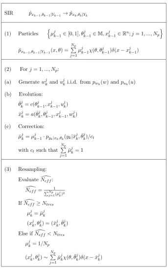
Table 2 gives an overview of the SIR particle filter cycle for the model in section 6.1. This table is based on table 1 in section 5. Only the evolution step in table 2 is different from the evolution step in table 1. In table 2, χ(θ, θj_k₋₁) is a 0−1 indicator with χ(θ, θj_k₋₁) = 1 ifθ=θj_k₋₁. Note thatpyk|xk,θk(yk|¯x

j k,θ¯

j

k) is the likelihood of the measurement at moment k

(40)

[image:40.595.130.474.126.673.2]

Table 2: SIR Particle Filter (SIR PF) cycle; state dependant on θk−1 and θk.

SIR p˜_x_k₋₁_,θ_k₋₁|Yk−1 →p˜xk,θk|Yk

(1) Particles nµj_k₋₁∈[0,1], θ_kj₋₁ ∈_M, xj_k₋₁ ∈_Rn_;_j_{= 1}_{, ..., N} p

o

˜

p_x_k₋₁_,θ_k₋₁|Yk−1(x, θ) =

Np

P

j=1

µj_k₋₁χ(θ, θj_k₋₁)δ(x−xj_k₋₁)

(2) For j= 1, ..., Np:

(a) Generatewj_k and uj_k i.i.d. from pwk(w) and puk(u)

(b) Evolution:

¯

θj_k=c(θ_kj₋₁, xj_k₋₁, uj_k)

¯

xj_k =a(¯θj_k, θ_kj₋₁, xj_k₋₁, wj_k)

(c) Correction:

¯

µj_k=µj_k₋₁·pyk|xk,θk(yk|¯x

j k,θ¯

j k)/ct

withct such that Np

P

j=1

¯

µj_k= 1

(3) Resampling:

Evaluate N[ef f:

[

Nef f = PNp1

j=1(¯µ j k)2

IfN[ef f ≥Ntres

µj_k= ¯µj_k

(xj_k, θ_kj) = (¯xj_k,θ¯_kj)

Else if N[ef f < Ntres

µj_k= 1/Np

(xj_k, θj_k)∼

Np

P

j=1

¯

(41)

6.3 Hybrid Particle filter for a system with state depending on θk−1 and θk

The Hybrid Particle filter (HPF) usesNp/M particles per mode, thus the amount of particles

per mode stays the same [Blom & Bloem, 2007; Blom & Bar-Shalom, 2009]. Whereas SIR particle filter could have very few particles in one mode at a certain time, when that mode has very few weight. For the investigation of the conditional densities per mode it is convenient if there are enough particles in every mode at every time step to get a good estimation of the conditional density.

The HPF is an extension of the SIR particle filter with a modified set of particles. That is, the total amount of particles per mode is constant. It seems plausible that for Np → ∞the

(42)

Table 3: Hybrid Particle Filter (HPF) cycle; state dependant onθk and θk+1.

HPF p˜_x_k₋₁_,θ_k₋₁|Yk−1 →p˜xk,θk|Yk

(1) Particles nµθ,j_k₋₁ ∈[0,1], xθ,j_k₋₁∈_Rn_{, θ}_∈

M,;j = 1, ..., Np/M

o

˜

p_x_k₋₁_,θ_k₋₁|Yk−1(x, θ) =

Np/M

P

j=1

µθ,j_k₋₁δ(x−xθ,j_k₋₁)

(2a) Mode switching:

uθ,j_k₋₁∼puk(u)

¯

θ_kθ,j =c(θ, xθ,j_k₋₁, uθ,j_k )

(2b) Prediction:

w_kθ,j ∼pwk(w) i.i.d., θ∈M, j∈ {1, ..., Np/M}

¯

xθ,j_k =a(¯θ_kθ,j, xθ,j_k₋₁, wθ,j_k )

(2c) Correction:

µθ,j_k =µθ,j_k₋₁·pyk|xk,θk(yk|¯x

θ,j k ,θ¯

θ,j k )/ct

withct such that Np/M

P

j=1

P

θ∈M

µj_k= 1

(3) Resampling:

γk(θ) = Np/M

P

j=1

P

η∈_M

µθ,j_k χ(¯θη,j_k , θ)

µθ,j_k =γk(θ)M/Np

xθ,j_k ∼

Np/M

P

j=1

P

η∈M

µθ,j_k χ(θ,θ¯η,j_k )δ(x−x¯θ,j_k )/γk(θ)

(43)

7 Generalized Interacting Multiple Model (IMM) algorithm

Following [Blom, 1985; 1986] the filtering problem considered addresses jump linear systems with jumps1 inx which occur simultaneously with and due to jumps in θ. Let {xk, θk}be a

two-component Markov process, with{xk}an Euclidean valued stochastic process and{θk}a

discrete valued process. The system considered satisfies a hybrid stochastic dynamical model of the form:

xk=A(θk, θk−1)xk−1+B(θk, θk−1)wk+C(θk, θk−1) (82)

where {wk} is a zero mean, Gaussian white noise process with covariance Q. Further,

{θk} is an M-valued Markov chain with transition probability matrix Π with components πθη=p{θk+1=η|θk =θ}. Letx∈Rn,θ∈M and w∈Rn

0

.

Consider the process{yk} which observes the process{xk}, according to the following

equa-tion:

yk=H(θk)xk+G(θk)vk (83)

where{vk}is a sequence of i.i.d. standard Gaussian variables of dimension m0 and

indepen-dent ofwk and y∈Rm.

The filtering problem is to estimate the joint conditional densityp_x_k_,θ_k|Yk(x, θ),x∈R

n_,_θ_∈

M,

of the pair (xk, θk) given Yk={ys;s≤k}, i.e. the realization of the process {yk}up to and

including momentk.

7.2 Generalized IMM algorithm for jump linear system with hybrid jumps

Following Blom [1986] it is assumed that for allj ∈_M the matricesA,B and C permit the following representation,

A(i, j) = A1(i)A2(i, j) (84) B(i, j) =

A1(i)B2(i, j) B1(i)

(85)

C(i, j) =

A1(i)C2(i, j) C1(i)

(86)

such that for alli∈_M A2(i, j),B1(i, j)B1(i, j)T and C1(i, j)C1(i, j)T are diagonal matrices.

Using (84), (85) and (86), equation (82) can be decomposed in two equations [Blom, 1986]:

xk = A1(θk)zk−1+B1(θk)w00k+C1(θk) (87)

zk−1 = A2(θk, θk−1)xk−1+B2(θk, θk−1)wk0 +C2(θk, θk−1) (88)

(44)

andw0_k w_k00T =wk.

The generalized IMM algorithm for the filtering problem in section 7.1, withC= 0 is described in [Blom, 1986] and [Blom, 1985]. This generalized IMM algorithm for the filtering problem in section 7.1 consists of time extrapolation equations betweenk−1 andkand measurement update equations on moment k. These equations are for the scalars pk(i), thendimensional

vectors ˆxk(i) and then×ndimensional matricesRk(i), which are for all i∈M the statistics

of approximations of pθk|Yk(i) and pxk|θk,Yk(x|i) in the following way:

pθk|Yk(i)

∼

= pˆk(i) (89)

p_x_k|θk,Yk(x|i)

∼ =

Z

x∈Rn

N_ˆ_x_k(_i₎_,_R_ˆ_k(_i₎(x)dx (90)

where NE,V is a Gaussian distribution on Rn with parametersE and V.

The time extrapolation equations from k−1 to kare:

Step I. Jump extrapolation equations for all i∈M follow from (88).

ˆ

zk−1(i, j) = A2(i, j)ˆxk−1(j) +C2(i, j) (91)

ˆ

Zk−1(i, j) = A2(i, j) ˆRk−1(j)AT2(i, j) +B2(i, j)B2T(i, j) (92)

¯

pk(i) =

X

j∈M

πjipˆk−1(j) (93)

¯

zk−1(i) =

X

j∈_M

πjipˆk−1(j)ˆzk−1(i, j)/p¯k(i) (94)

¯

Zk−1(i) =

X

j∈M

πjipˆk−1(j){Zˆk−1(i, j) + [ˆzk−1(i, j)−z¯k−1(i)].[ˆzk−1(i, j)−z¯k−1(i)]T}/p¯k(i)

(95)

Step II.Kalman time extrapolation equations for alli∈_M follows from equation (87).

¯

xk(i) = A1(i)¯zk−1(i) +C1(i) (96)

¯

(45)

Step III.Measurement update equations for alli∈_M at moment k.

vk(i) = yk−H(i)¯xk(i) (98)

Qk(i) = H(i) ¯Rk(i)H(i)T +G(i)G(i)T (99)

Kk(i) = R¯k(i)H(i)TQk(i)−1 (100)

ˆ

xk(i) = x¯k(i) +Kk(i)vk(i) (101)

ˆ

Rk(i) = R¯k(i)−Kk(i)H(i) ¯Rk(i) (102)

ˆ

pk(i) = ckp¯k(i)kQk(i)k−

1

2 exp{−1

2v

T

k(i)Qk(i)−1vk(i)} (103)

withck a constant such that

P

i∈_M

ˆ

(46)

(47)

8 Target motion models

8.1 Target motion model with two modes

We look at a target motion model for one axis of motion. This model describes the dynamics of an object moving on a straight line, i.e. a one-dimensional space. The object’s possible movements are considered to be constant speed and acceleration. The acceleration in this case can be positive or negative. The model and parametrization is from [Blom & Bloem, 2007].

Consider the following one-dimensional motion model:

x=sx s˙x ¨sx

T

(104)

with sx the target position, ˙sx the groundspeed and ¨sx the target acceleration.

Consider also a two-component Markov process {xk, θk} with {xk} an Euclidean valued

stochastic process and{θk}a discrete valued process.

The system considered satisfies a hybrid stochastic dynamical model of the form:

xk+1=A(θk+1)xk+B(θk+1)wk (105)

wherewk is a sequence of i.i.d. standard Gaussian variables of dimension one.

The process of switching between the different movements is represented by an M-valued

Markov chain {θk}. M is the set of discrete modes. In this case M = {0,1}. With θk = 0

representing the object moves with constant speed and withθk = 1 representing the object

is accelerating (or decelerating). The Markov chain{θk} has transition probability matrix Π

with componentsπθη = p{θk+1 = η|θk = θ}. The following transition probability matrix Π

will be used for the Markov chain{θk}:

Π = 

 1− ts

τ1

ts

τ1

ts

τ2 1−

ts

τ2



 (106)

For A(θ) we have:

A(0) = 



1 ts 0

0 1 0

0 0 0



 A(1) =





1 ts 1₂t2s

0 1 ts

0 0 α



 (107)

where ts is the sampling time interval and the parameter α ∈ (0,1] allows the acceleration

(48)

appendix B.

ForB(θ) we have:

B(0) =σa

  0 0 1 

 B(1) =σa

p 1−α2

  0 0 1   (108)

whereσa represents the standard deviation of the acceleration noise.

Consider the process{yk}which observes the statexk. The process{yk}satisfies the following

equation:

yk = Hxk+σmvk (109)

whereH=1 0 0and vk is a sequence of i.i.d. standard Gaussian variables of dimension

one independent ofwk. σm represents the standard deviation of the measurement error.

8.2 Target motion model with three modes

We look at a target motion model for one axis of motion. This model describes the dynamics of an object moving on a straight line, i.e. a one-dimensional space. The objects possible movements are considered to be constant speed, positive acceleration and negative accelera-tion. The model is a three modes version of the two modes example in [Blom & Bloem, 2007]. Note that this model makes a distinction between positive and negative acceleration whereas the model in section 8.1 considers positive and negative acceleration as one mode.

Consider the following one-dimensional motion model:

x=

sx s˙x ¨sx

T

(110)

with sx the target position, ˙sx the groundspeed and ¨sx the target acceleration.

Consider also a two-component Markov process {xk, θk} with {xk} an Euclidean valued

stochastic process and{θk}a discrete valued process.

The system considered satisfies a hybrid stochastic dynamical model of the form:

xk+1 =A(θk+1, θk)xk+B(θk+1, θk)wk+C(θk+1, θk) (111)

wherewk is a sequence of i.i.d. standard Gaussian variables of dimension one.

The process of switching between the different movements is represented by an M-valued