Development of Predictive Control
Strategies for Building Climate
Control
Himanshu Nagpal
Department of Civil, Structural & Environmental Engineering
University of Dublin
This dissertation is submitted for the degree of
Doctor of Philosophy
Declaration
I declare that this thesis has not been submitted as an exercise for a degree at this or any other university and it is entirely my own work. I agree to deposit this thesis in the University’s open access institutional repository or allow the library to do so on my behalf, subject to Irish Copyright Legislation and Trinity College Library conditions of use and acknowledgement.
Acknowledgements
First of all I would like to pay my deepest gratitude to my supervisor Prof. Biswajit Basu for his enlightening guidance throughout this journey. Without his support this thesis would not have been possible. I feel he believed in me during the times when I had lost self-belief. For this I am most grateful.
Special thanks to Dr. Andrea Staino and Dr. Lin Chen for their valuable sugges-tions and comments on part of this research work. This research was funded by the European Commission under the projects INDICATE (FP7) and EINSTEIN (Marie Curie actions), which is highly acknowledged.
Abstract
The rapid growth in energy usage and CO2emissions has become a critical issue
for the whole world. It is noteworthy that buildings are a major contributor to global primary energy consumption. Among building services, use of energy in heating-ventilation-air-conditioning (HVAC) system is particularly significant (about 50% of the total building energy consumption). Therefore, the development and implementation of effective control strategies to optimize the operation of HVAC systems in context of energy usage is essential. One such class of advanced control approaches is model predictive control (MPC). The fundamental idea behind MPC is to use the dynamical model of the process (thermal environment of building in this case) to predict its evolution and optimize the control input signal based on those predictions.
The first part of this thesis provides a detailed introduction to MPC and is devoted to studying the application of MPC in the context of building energy system and climate control.
vi
The remaining part of the thesis is dedicated to the design of advanced robust MPC controllers to control indoor building environment. These controllers pro-vide robustness against uncertainties present in the system which may arise due to various reasons like plant model mismatch, uncertain system gain and/or ad-ditive external disturbances. The robust MPC controller presented in this thesis is intended to handle uncertainty in the thermal model of the building and also additive bounded disturbances to the systems mainly from solar irradiance and ambient temperature.
Table of contents
List of figures xi
List of tables xv
1 Introduction 1
1.1 Building Energy Overview . . . 1
1.2 HVAC System and Control . . . 2
1.2.1 Classical Control Techniques . . . 2
1.2.2 Modern Control Techniques . . . 4
1.3 Literature Review and Discussion . . . 5
1.4 Contribution of The Thesis . . . 10
1.5 Outline of The Thesis . . . 11
2 Model Predictive Control 12 2.1 Dynamical Model Representation . . . 12
2.1.1 Linear Time-Variant (LTV) System . . . 13
2.1.2 Linear-Time Invariant (LTI) System . . . 14
2.1.3 Discrete Time State-Space Model . . . 14
2.2 MPC strategy . . . 14
2.3 Mathematical Formulation . . . 15
2.3.1 Objective Function . . . 15
2.3.2 Constraints . . . 18
Table of contents viii
2.5 Infinite Horizon MPC . . . 19
2.6 Model Identification . . . 20
2.6.1 White-box System Identification . . . 20
2.6.2 Black-Box System Identification . . . 20
2.6.3 Grey-Box System Identification . . . 21
3 Building Thermal Environmental Control and MPC 22 3.1 Building Description and Thermal Model Formulation . . . 23
3.2 Formulation of Optimization Problem . . . 26
3.3 Weather Forecast . . . 28
3.3.1 Recursive ARIMA modelling . . . 29
3.4 Forecasting using Recursive Seasonal ARIMA . . . 30
3.5 Seasonal Arima Model . . . 31
3.6 Simulation Setup and Results . . . 34
3.7 Summary . . . 37
4 Model Predictive Control with Cooperative Optimization Framework 38 4.1 Cooperative Optimization framework . . . 38
4.2 Concept of MPC with Cooperative Optimization Framework . . . 41
4.3 Simulation Setup and results . . . 42
4.3.1 Selfish Optimization . . . 44
4.3.2 Cooperative Optimization . . . 47
4.4 Summary . . . 52
5 Robust MPC with Uncertainty in Building Parameters 53 5.1 Model with Polytopic Uncertainty . . . 54
5.2 Synthesis of Robust Controller . . . 55
5.2.1 Robust Constraint MPC . . . 55
5.2.2 Reference Trajectory Tracking . . . 58
Table of contents ix
5.4 Simulation Results . . . 60
5.4.1 Effects of model uncertainty . . . 60
5.4.2 Robust MPC in presence of uncertainty . . . 61
6 Approximate Close-loop Minimax MPC with Bounded Additive Distur-bances 66 6.1 Previous Work and Motivation . . . 67
6.2 Uncertainty Model . . . 67
6.3 Minimax MPC . . . 69
6.4 Problem Formulation . . . 71
6.5 Simulation Setup and Results . . . 72
6.6 Summary . . . 74
7 Energy management in a Residential Building using Mixed Integer Linear Programming with Real-Time Pricing 76 7.1 Load Categorization . . . 76
7.1.1 Thermal load . . . 77
7.1.2 Non-thermal load . . . 77
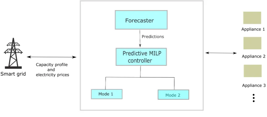
7.2 System Architecture . . . 77
7.3 Appliances Modelling and Setup . . . 78
7.3.1 State-space model . . . 78
7.3.2 Thermal Appliances Modelling . . . 79
7.4 Non-thermal Appliances Modelling . . . 80
7.5 Problem Formulation and Scheduling Algorithm . . . 81
7.5.1 Problem Formulation . . . 81
7.5.2 Scheduling algorithm . . . 84
7.6 Simulation Studies . . . 84
7.6.1 Simulation setup . . . 84
7.6.2 Simulation results . . . 87
Table of contents x
8 Conclusions and Future Work 93
List of figures
2.1 MPC strategy . . . 16
2.2 Basic design of MPC . . . 17
2.3 Black-box system identification . . . 21
3.1 Residential building modeled in IES-VE . . . 24
3.2 RC schematic of simplified building thermal model . . . 24
3.3 Estimation of indoor temperature using IES-VE and reduced order model (ROM) . . . 26
3.4 Ambient temperature data used for recursive ARIMA forecasting . . 32
3.5 Solar irradiance data used for recursive ARIMA forecasting . . . 32
3.6 Comparison between simulated temperature using recursive ARIMA and real temperature data . . . 33
3.7 Prediction error of temperature data with recursive ARIMA approach 33 3.8 Comparison between simulated irradiance using recursive ARIMA and real irradiance data . . . 34
3.9 Prediction error of irradiance data with recursive ARIMA approach . 34 3.10 Zone temperature dynamics of the building . . . 36
3.11 Power input from HVAC to the building . . . 36
4.1 Group ofnbuildings connected tomheat-pumps . . . 39
List of figures xii
4.3 Power consumption of heat-pump for small building with selfish optimization . . . 45 4.4 Indoor temperature dynamics for large building with selfish
optimiza-tion . . . 46 4.5 Power consumption of heat-pump for large building with selfish
optimization . . . 46 4.6 Indoor temperature dynamics for office building with selfish
opti-mization . . . 47 4.7 Power consumption of heat-pump for office building with selfish
optimization . . . 48 4.8 (a) Indoor temperature dynamics for small building with cooperative
optimization, (b) Indoor temperature dynamics for large building with cooperative optimization . . . 49 4.9 (a) Power consumption of heat-pump for small building with
coop-erative optimization, (b) Power consumption of heat-pump for large building with cooperative optimization (c) Total Power consumption of heat-pump for both buildings with cooperative optimization . . . 49 4.10 Total power consumption for both residential buildings with selfish
and cooperative optimization . . . 50 4.11 (a) Indoor temperature dynamics for small building with cooperative
optimization, (b) Indoor temperature dynamics for office building with cooperative optimization . . . 51 4.12 (a) Power consumption of heat-pump for small building with
cooper-ative optimization, (b) Power consumption of heat-pump for office building with cooperative optimization (c) Total Power consumption of heat-pump for both buildings with cooperative optimization . . . 51 4.13 Total power consumption for office and small residential building
with selfish and cooperative optimization . . . 52
List of figures xiii
5.2 Effect of parametric uncertainty on nominal MPC corresponding to 50% variations in the parameters . . . 62 5.3 Performance deterioration of nominal MPC with variations in
param-eters . . . 62 5.4 Zone temperature and control input evolution corresponding to a
corner point of the polytopeΩ. . . 63
5.5 Effect of uncertainty on nominal MPC in presence of uncertainty with sinusoidal variation ofλ . . . 64
5.6 Indoor temperature trajectory and the heating input for robust MPC with sinusoidal variation ofλ . . . 65
5.7 Performance error comparison of robust and nominal MPC with sinusoidal variation ofλ . . . 65
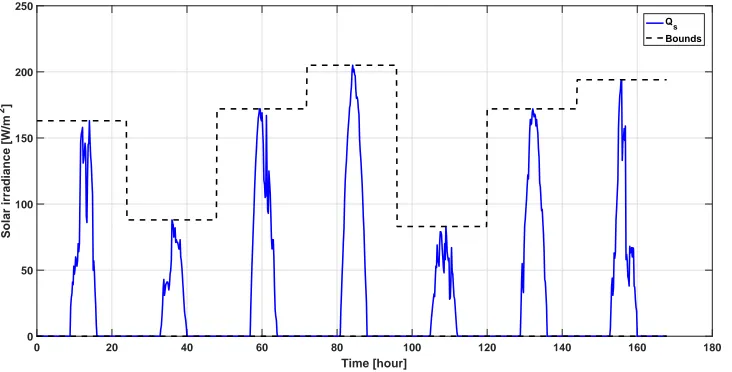
6.1 Derived bounds on ambient temperature . . . 72 6.2 Derived bounds on solar irradiance . . . 73 6.3 Zone temperature dynamics of the building with no knowledge of
disturbance . . . 74 6.4 Zone temperature dynamics of the building with additive bounded
disturbance with close-loop minimax MPC . . . 74 6.5 Heating input power consumption of HVAC with close-loop minimax
MPC . . . 75 6.6 Heating input power consumption of HVAC with close-loop minimax
MPC . . . 75
7.1 System architecture of HEMS . . . 78 7.2 Algorithm used for scheduling of appliances . . . 85 7.3 (a)Room temperature with HEMS, (b)Power consumption by heat
pump with HEMS . . . 88 7.4 (a) Temperature of water in water tank with HEMS, (b) Power
List of figures xiv
7.5 (a) Power consumption of washing machine with HEMS, (b) Power consumption of dishwasher with HEMS . . . 90 7.6 (a) Total power consumption of household appliances with HEMS,
List of tables
3.1 Description of model parameters . . . 27
3.2 Description of model parameters . . . 35
7.1 Description of parameters involved in equation (7.2) . . . 79
7.2 Description of parameters involved in equation (7.3) . . . 80
7.3 Thermal appliance parameters . . . 86
Chapter 1
Introduction
The rapid growth in energy usage and related CO2emissions has become a critical
issue for the whole world. According to the data gathered by International Energy Agency, the world’s primary energy consumption has grown by 102%, and CO2
emissions have increased by 108% during the last four decades (1973-2017); which is evidently a prime concern for the global economy and environment [24]. Therefore, appropriate measures must be taken to handle this issue.
1.1
Building Energy Overview
1.2 HVAC System and Control 2
While discussing building energy, one important factor to be considered is build-ing energy efficiency which indicates the ratio of the output of energy, performance and service of the building to the on-site energy consumption. The energy effi-ciency in buildings can be enhanced by achieving desired output with the use of less amount of energy leading to an improved performance of the building. As a matter of fact, the buildings sector is consistently recognized as a primary potential area of achieving better energy efficiency [23].
1.2
HVAC System and Control
As mentioned previously, HVAC system services are the major source of energy con-sumption in buildings. Therefore, the development and implementation of effective control strategies for HVAC system are essential. In particular, with the technological advancement of information and communication services and reduced cost of data storage and processing in recent years, it has become feasible to implement sophisti-cated control strategies into building energy systems. Based on a comprehensive review about theory and application of control in HVAC presented in [4], the control aspects of HVAC are discussed below.
1.2.1
Classical Control Techniques
In the literature, many approaches for the control of HVAC systems exist. From a practical point of view on/off control, proportional integral derivative (PID) and weather compensated control are the most commonly used approaches due to their simplicity. However, these control strategies result in a compromised performance of HVAC system.
On/Off Control
1.2 HVAC System and Control 3
turned on or off according to the deviation from a setpoint, i.e., based on an error threshold. When the indoor temperature is below the lower threshold, the heating system turns on, and when the indoor temperature is above the upper threshold, the heating system turns off. The controller does not consider the building’s thermal dynamics at all. Although, On/Off control is simple and intuitive to design, it is not capable of handling processes with time delays and provide minimal authority to the user in terms of energy efficiency.
Weather Compensated Control
Weather compensated control is a feedforward form of control. A sensor is placed outdoor to provide information about external ambient temperature to the controller regularly. As the outdoor temperature changes, the heating system responds to that change according to a predefined heating curve thus altering the indoor temperature. This curve is a function of the difference between the internal and the external temperature. This controller also doesn’t account for the dynamics of the building.
PID control
1.2 HVAC System and Control 4
1.2.2
Modern Control Techniques
The controllers strictly based on the theory of control systems are included in this division. Most common examples are gain scheduling control, optimal control, Lyapunov based nonlinear control and model predictive control.
Gain Scheduling Control
Gain scheduling control is a popular approach used to control the systems whose dy-namics depend on one or morescheduling variablelike system parameters, operating conditions and time. The nonlinear system is decomposed into linear subsystems based on the scheduling variable, and for each subsystem, a linear controller is designed appropriately.
Nonlinear Feedback System Control
Nonlinear control is a well-developed area of control theory due to the existence of nonlinearity in most real-world systems. Rigorous mathematical techniques have been developed to analyze nonlinear systems which include Lyapunov stability analysis, describing functions and center manifold theorem. The control law can be obtained by using feedback linearization and other Lyapunov based control techniques.
Optimal Control
1.3 Literature Review and Discussion 5
Model Predictive Control
Model predictive control (MPC) is an advanced control strategy which has been widely applied in the process control industry since the 80’s. MPC includes a class of control strategies where the dynamical model of the process is considered to predict the evolution of the process, and an optimized control input signal is derived based on those predictions.
MPC has several inherent advantages over other control techniques
• MPC uses a model of the process to determine the optimized control actions based on explicitly predicted behavior of the process;
• A disturbance model can be integrated into the process model itself to account for disturbance rejection;
• The approach is suitable with multi-input-multi-output (MIMO) processes too;
• Constraints can be incorporated on control variables as well as on state vari-ables easily; even time-varying constraints can be imposed conveniently ;
• The technique is well-suited for slow dynamics processes with time delay, e.g. building thermal environment.
MPC and its application in building climate control will be discussed later in the thesis.
1.3
Literature Review and Discussion
1.3 Literature Review and Discussion 6
There is a basic standard structure to design MPC based on which, various strategies have been proposed in the literature. The key difference between different techniques is the objective of the control system. Most often, MPC is designed with the intention of providing better regulation of temperature [44], energy demand reduction by load shifting [9, 49], minimizing energy usage [38, 28] and electricity cost savings [35, 17, 60, 36]. Moreover, MPC has been implemented with a focus on various other objectives like minimizing computation needs and faster operation time [64], better indoor air quality [59] and disturbance rejections [21, 62] etc.
In the study carried out by authors in [38], a library building is considered at the University of California, Berkeley. The thermal model of the building is developed using lumped-capacitance method and validated using real air temperature data. The internal and external load is parametrized as a function ofCO2concentration in
the building and external weather conditions. A bilinear model is extracted using a non-linear regression technique and linearized at the nearest equilibrium point. The objective function is expressed as linear combination of total energy consumption and peak air-flow. The simulation is performed using YALMIP with Matlab. As a result, a reduction of 33% in peak air-flow rate and 73% in total energy consumption in comparison to the original controller is achieved.
1.3 Literature Review and Discussion 7
An experimental study is carried out in [37], in which the target building (Uni-versity of California, Mercedes campus) is equipped with a water tank to act as heat storage. An optimal thermal energy storage strategy is developed using MPC. A so-lar load predictor is employed to capture the external thermal load based on position of the sun at current time/date, building geometry and cloud coverage. The internal thermal load is expressed as a piecewise constant periodic signal with a period of one week. Further, based on the internal and external load, the total thermal load of the building is predicted by modelling the building using a resistance- capacitance (RC) circuit method. The parameters of the building thermal model are identified using historical data by minimizing the thermal model output and measured load on the campus. The optimization problem is formulated as mixed integer non-linear programming (MINLP) problem. The system is operated under three different sce-narios to compare the efficacy of the proposed MPC. The performance of the system is evaluated based on electricity bill and coefficient of performance (COP) of the plant. The results showed significant reduction in electricity bill information and the COP is increased by 11.9%.
Another experimental case study was done in [54] at the Czech Technical Uni-versity in Prague. The building is considered with two heating circuit and two reference rooms. The thermal dynamics of the rooms are captured using an RC circuit technique. The parameters of the rooms are estimated using stochastic dif-ferential equation with maximum likelihood method. The objective of the control system is to minimize the energy consumption and to track a pre-specified reference trajectory. The problem is implemented in Scilab and the optimization problem is solved using an internal linear-quadratic (LQ) solver from SciLab. The results demonstrated that energy savings of 15% to 28% (depending on various factors) is achieved using MPC.
1.3 Literature Review and Discussion 8
vector regression (SVR) method is used to obtaing simplified dynamical model of the HVAC system. The design parameters of support vector machine (SVM) is tuned to fit the measured temperature data of the building. The objective function is expressed as combination of thermal comfort, power consumption and the rate of power usage. The non-linear optimization problem is solved using iterative dynamic programming.
Another noteworthy work is accomplished where the thermal comfort of oc-cupants of the building is explicitly considered into the objective function using predicted mean vote (PMV) index [11]. In [52], MPC is used with exact feedback lineariation for temperature control by water-to-air heat exchangers in HVAC sys-tem. An implicit variation of the MPC strategy can be noticed based on a different approach to solve the optimization problem [62, 28]. A detailed literature review on the theory and applications of MPC is also available [4].
There are few studies on MPC in the context of uncertainty [39, 47, 48, 68]. In [47], a simulation study is performed using stochastic model predictive control (SMPC) to achieve desired thermal comfort. In order to consider uncertainties in weather predictions, the constraints are enforced to be fulfilled with a predefined probability. Affine disturbance feedback is used to formulate the resulting problem as a convex optimization problem. A performance bound is defined as optimal control with perfect knowledge of the system dynamics and future disturbances which act as a theoretical benchmark for the proposed control strategy. The weather forecast is expressed as sum of weather forecast delivered by MeteoSwiss [58] and the prediction error. The predictions are updated every 12 hours using a Kalman filter. A probabilistic cost function is used with the aim of minimizing the expected value of energy usage. The approach can be generalised to account for uncertainty in occupancy predictions also.
un-1.3 Literature Review and Discussion 9
certainty is modelled using an autoregressive model. The thermal dynamics of the building are modelled as a twelfth order bilinear model. The constraints are formulated as chance constraints similar to SMPC. In this approach, random convex programs are solved when uncertainty is fixed. The results showed that RMPC outperforms the compared methods and deals with non-additive and non-Gaussian uncertainties.
An interesting experimental study is done in [39] where the emphasis is on handling the model uncertainties. The target building in the study is an office building in Lakeshore building at the Michigan Technological University. The building uses a ground source heat pump for heating purposes. In this work, a novel parameter adaptive building (PAB) model is proposed and developed which allows an online and automatic parameter estimation of the building. The thermal dynamics of the building is modelled using an RC circuit method. In order to estimate the parameters of the building, an extended Kalman filter is used. The objective of the control system is to minimize energy consumption and maintain thermal comfort. The results demonstrated that the proposed approach is able to achieve the objective in presence of model uncertainties up to 70%. However, since the parameters of the building are estimated at each time step, implementation of the control command may be computationally inefficient. Further, the approach is heavily dependent on the accuracy of the parameters identified, which may have an impact on the performance of the controller.
1.4 Contribution of The Thesis 10
1.4
Contribution of The Thesis
Based on the literature review, the following gaps in the literature are identified,
• Most of the approaches reported in the literature mainly investigate energy performance and efficiency in individual buildings. Therefore, further research on building energy performance for a group or cluster of buildings is necessary to achieve energy efficiency at a district or city level.
• The research work in the field of HVAC control with MPC accounting for uncertainties is still limited. The proposed approaches are either computation-ally expensive or practiccomputation-ally inefficient. Roust control strategies for building climate control have not been studied thoroughly yet and have not received the attention they deserve.
In accordance with the identified gap in the literature, the following main ideas are addressed in the thesis
• The control of HVAC system for a cluster of buildings is investigated and a novelcooperative optimizationframework to is proposed to enhance energy performance of the cluster.
• A new robust control scheme for building thermal environment is formulated that is capable of handling uncertainties in the thermal model description of the building.
• Next, a new HVAC system control scheme is proposed which is designed to provide robustness against additive disturbances to the system like solar gain and ambient temperature.
1.5 Outline of The Thesis 11
1.5
Outline of The Thesis
Chapter 2
Model Predictive Control
This chapter is provides a brief introduction to model predictive control (MPC) theory. MPC is an advanced control approach which can be traced back to late 1970’s to early 1980’s in the process industry and has been developed significantly since then. In the literature, MPC refers to a class of control strategies where the dynamical model of the process is explicitly considered to predict future behaviour of the system and control input is derived based on the optimization of a performance criterion with certain constraints on the states and control variables.
2.1
Dynamical Model Representation
As mentioned, the dynamical model of the process is involved in deriving the control law, so an appropriate model of the process is necessary to capture the dynamics and behaviour of the system. There exist various descriptions and formulations of the process model. For example- Impulse Response (IR) model, Transfer Function (TF) model, State-Space (SS) model, etc.
2.1 Dynamical Model Representation 13
A dynamical system can be generally described in state-space form by the fol-lowing differential equation
dx(t)
dt = f(x(t),u(t),w(t),t) y(t) =g(x(t),u(t),t)
x(t0) =x(0)
(2.1)
wherex∈Rnis the state vector,u∈Rmis the control input vector,y∈Rprefers to the output vector of the system andw∈Rr represents the external disturbance vector acting upon the system andt∈Ris the time.x(t0)is the state of the system at initial
timet0.
The system described in equation (2.1) is nonlinear, i.e., the evolution of the system states is a nonlinear function of time. For simplicity, the work in this thesis is restrained to linear dynamical systems only.
2.1.1
Linear Time-Variant (LTV) System
The linear time-variant system in continuous state-space form is represented as following
dx(t)
dt =A(t)x(t) +B(t)u(t) +E(t)w(t) y(t) =C(t)x(t) +D(t)u(t)
x(t0) =x(0)
(2.2)
A∈Rn×nis the dynamics or state-transition matrix,B∈Rn×mis the control or input
matrix, C ∈Rp×n is the output matrix, D∈Rp×m is the feedthrough matrix and
E∈Rn×r is the disturbance matrix. It should be noted that these system matrices are
2.2 MPC strategy 14
2.1.2
Linear-Time Invariant (LTI) System
Linear-time-invariant systems in continuous state-space form is expressed as
dx(t)
dt =Ax(t) +Bu(t) +Ew(t) y(t) =Cx(t) +Du(t)
x(t0) =x(0)
(2.3)
Notice here the system matrices are fixed and do not depend upon time.
2.1.3
Discrete Time State-Space Model
This model representation is used in the processes which involve empirical or sensory measurements. The discrete time state-space model of a system is described as following
xk+1=Axk+Buk+Ewk
yk=Cxk+Duk
x0=x(0)
(2.4)
Here k represents the time step at which computations and measurements are performed. In this thesis, this representation to model the systems has been used.
2.2
MPC strategy
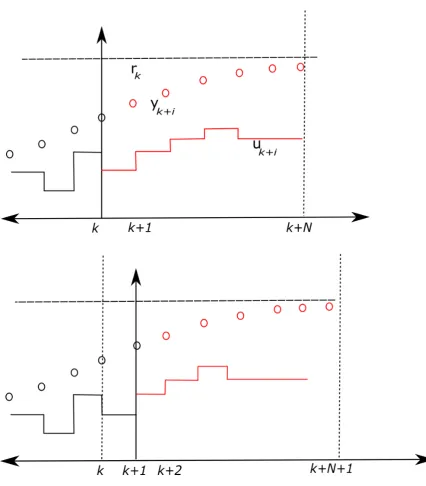
All the approaches belonging to the MPC class have following characteristics, repre-sented in figure 2.1:
• At each time step k, the future output of the process yk+i|k, i=1,2. . .N is
2.3 Mathematical Formulation 15
control input signalsuk+i|k, i=0,1, . . .N−1. These future control input signals
are calculated by optimizing certain performance criterion.
• The control input signal uk|k is applied to the process while the rest control
inputs are discarded. At the next time stepk+1, the new state of the system
xk+1is known already, and the same procedure of output prediction and control
action calculation is repeated with the new information available.
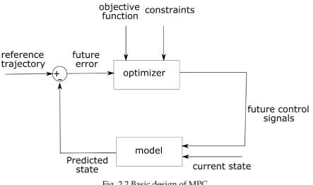
The basic design of above strategy is represented in figure 2.2. A dynamical model is used to predict the future states of the process, based on the current state and future control signals. The future control signals are obtained from an optimizer which optimizes a certain objective function considering the constraints imposed on the system state and control input to produce optimal control sequence. The prediction horizon represents the limit on the number of time step up to which the system states the system states would be predicted. Similarly, control horizon is the number of time step up to which the future control actions are calculated. The number of time steps considered for predictions is finite hence the above strategy is referred as
finite receding horizon controltoo. However, it is not always necessary to have a finite
prediction horizon rather it is seen in later section that the use of a finite horizon may lead to a compromise in the stability of the control system.
2.3
Mathematical Formulation
In this section, the control strategy described in section 2.2 is formulated in math-ematical terms. To implement the control, first the objective function need to be defined based on which the control inputs will be derived.
2.3.1
Objective Function
2.3 Mathematical Formulation 16
2.3 Mathematical Formulation 17
Fig. 2.2 Basic design of MPC
system using the appropriate mathematical function. The objective function could be linear (e.g., economic MPC), quadratic (e.g., nominal MPC) or even nonlinear depending upon the control problem.
For now, the task of tracking a certain reference trajectory at minimal input cost is considered. For a system presented in equation (2.4), the objective functionJfor tracking problem can be written as following
J=
N
∑
i=1
(xi+k−ri)TQ(xi+k−ri) +uTi+kRui+k+xTN+1SxN+1 (2.5)
where N is the prediction horizon. Q and R are positive semi-definite and posi-tive definite weighting matrices associated with system states and control inputs respectively. The term on far right end is the terminal state penalty cost with S as the weighting matrix. ri represents the reference value after itime steps. It is
2.3 Mathematical Formulation 18
trajectory is known in advance which gives flexibility to the system to react a priori thus avoiding time-delay effects.
2.3.2
Constraints
Almost every real world dynamical system (car driving, stirred tank system, power system etc.) is subjected to constraints . As such, the control action which actuates the process should rest in a certain range, and similarly, the states of the system should be kept within a permissible limit. The system states and control input sequence need to satisfy
xK ∈X
uk∈U (2.6)
where Xis a convex, closed subset ofRn andUis a convex, compact subset ofRm and each set contains the origin in the interior of the set. In general, constraints are treated in two ways in MPC
Soft Constraints
In a soft constraints formulation, the constrained variable is allowed to violate the constraints at the cost of a large penalty. So, the controller appropriately decides to make a trade-off between constraint violation and the cost penalty. Usually, constraints on output variables are treated this way.
Hard Constraints
The constraints on control input are generally treated as hard constraints. In this constraint setting, the constrained variable can not violate the constraints.
2.4 Optimization 19
2.4
Optimization
To derive optimal control sequence, a optimizer minimizes the objective functionJ subjected to the constraints and system dynamics.
U∗=min
u N−1
∑
i=0
(xi+k−ri)TQ(xi+k−ri)+uTi+kRui+k+x(N)TSx(N) (2.7)
subjected to
xk+i+1=Axk+i+Buk+i i=0,1, . . .N−1 yk+i=Cxk+i+Duk+i i=0,1, . . .N−1
x0=x(0)
xmin≤xk+i≤xmax, i=0,1, . . .N−1
umin≤uk+i≤umax, i=0,1, . . .N−1
(2.8)
whereUi∗|Ni=1is the optimal control input policy which minimizes the error between
reference temperature trajectory and future states subjected to the system dynamics and imposed constraints. In other words, control input policyUi∗drives the system states to desired reference values. Evidently,xmin,xmax andumin, umax represents
the lower and upper bound on the permissible range of the system states and the control inputs. Only the first component of the optimal control law is implemented i.e. U1∗and obtain the system state xk+1 by applying this control input. Now the
new information is available about reference trajectory, constraints and disturbances (discussed later), so according to receding horizon control strategy this optimization procedure is repeated withxk+1as the current state of the system.
2.5
Infinite Horizon MPC
In 1960, Kalman in his paper [27] explained that ‘system with optimal control law is not
2.6 Model Identification 20
infinite horizon control law is stabilizing’. For infinite horizon MPC, the objective
function is formulated in the following form
J=
∞
∑
i=1
(xk+i−ri)TQ(xk+i−ri) +uTk+iRuk+i (2.9)
The use of infinite horizon ensures that the cost function J is Lyapunov which implicates the close loop stability.
2.6
Model Identification
The modelling and identification of systems, which describe the dynamics of the underlying processes is a wide area of research in itself. However, this section briefly overviews the approaches involved in the process of system identification.
2.6.1
White-box System Identification
In this system identification approach, the model of the system is derived from first principles. For example, a detailed model of the thermal dynamics of a building can be obtained by heat-balance equations, a physical model of a dynamical system can be captured using Newton’s laws of motion, or any fluid flow can be analysed using fluid dynamics equations. However, in many real-world cases, this approach may be difficult to use due to inherent complexities of the process.
2.6.2
Black-Box System Identification
2.6 Model Identification 21
2.3). The approach is widely used to derive models for nonlinear systems. However, the transparency of the process is compromised.
Fig. 2.3 Black-box system identification
2.6.3
Grey-Box System Identification
In this approach, a generic model of the process is available while granular details of the system dynamics may not be accessible. The parameters of the generic model are identified using available data about the process behaviour. The parameter can be estimated by manually calibrating the model to the data or by using some estimation algorithm or both. This approach involve a partial model of the process (white-box) and data-driven (black-box) identification both, hence it is referred as grey-box system identification.
Chapter 3
Building Thermal Environmental
Control and MPC
This chapter focuses on the application of MPC to HVAC systems. First of all, a simplified thermal model of a building attached to a simple HVAC system is presented using mathematical equations, and later an MPC controller is designed to maintain the indoor temperature close to certain reference setpoints. The key idea here is that the control system has advance information about the future weather conditions and reference setpoint trajectory. The building envelop can function as temporary heat storage to store energy and use it to meet thermal comfort demand.
3.1 Building Description and Thermal Model Formulation 23
3.1
Building Description and Thermal Model
Formula-tion
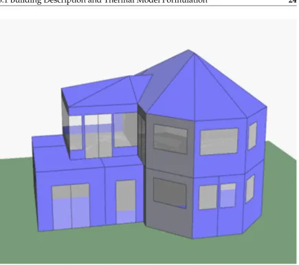
For control description, a residential building from a village in the north of Scotland is considered and modelled using building energy software IES-VE (see figure 3.1). This work has been conducted under project EINSTEIN by European Union The house considered is a two-storey dwelling, with a floor space of 160 m2 and 15 rooms. For simplification, a single-zone model of the building is considered for system identification of the reduced order model (ROM) without any loss of accuracy in simulating the states of interest. The RC (resistance-capacitance) schematic of the thermal model is provided in figure 3.2. The windows are assumed to have very little thermal mass and are modelled as a pure resistance term. The internal building mass includes floors, interior walls, ceilings, and furniture. The air within the building envelope is assumed to be fully mixed. The effect of the wind is not considered here. The thermal dynamics of the building can be captured in a mathematical form using heat-balance equations. The following simplified model is derived to represent the thermal behaviour of the building
Cp,zT˙z=−(UA)za(Tz−Ta)−(UA)z f(Tz−Tf)−hiAs(Tz−Tsi) +Qheat+Qs
Cp,s
2 T˙si=hiAs(Tz−Tsi) + ks
tsAs(Tse−Tsi)
Cp,s
2 T˙se=heAs(Ta−Tse) + ks
tsAs(Tse−Tsi)
Cp,fT˙f = (UA)z f(Tz−Tf)
(3.1)
3.1 Building Description and Thermal Model Formulation 24
[image:39.595.90.526.80.465.2]Fig. 3.1 Residential building modeled in IES-VE
3.1 Building Description and Thermal Model Formulation 25
The set of equations presented in equation (3.1) can be written in continuous time state-space model as per the equation (2.3).
dx(t)
dt =Ax(t) +Bu(t) +Ew(t) y(t) =Cx(t)
x(t0) =x0
(3.2)
wherex=hTz Tsi Tse Tf
iT
is the state vector,u=Qheat is the control input to the system,w=hWs Ta
iT
is the external disturbance acting on the system andy=Tzis
the output variable. The matrices in state-space model (3.2) are
A=
a11 a12 0 a14
a21 a22 a23 0
0 a32 a33 0
a41 0 0 a44
E=
e11 e12
0 0
e31 0
0 0 (3.3a)
C=h1 0 0 0i B=hC1
p,z 0 0 0 iT
(3.3b)
where
a11= (−(UA)za−C(UA)z f−hiAs)
p,z a12=
hiAs
Cp,z a14=
(UA)z f
Cp,z
a21= 2ChiAs
p,s , a22=
2(−hiAs−ktssAs)
Cp,s a23=2
ksAs
tsCp,s
a32=a23, a33= 2
(−heAs−ktssAs)
Cp,s a41 =
(UA)z f
Cp,f
a44=−a41 e11= (UAC )za
p,z
e12 =C1
p,z
e31= 2CheAs
p,s
3.2 Formulation of Optimization Problem 26
obtained
xk+1=Adxk+Bduk+Edwk
yk=Cdxk
(3.4)
[image:41.595.90.523.231.570.2]where subscriptdrefers to the discretized version of the system matrix.
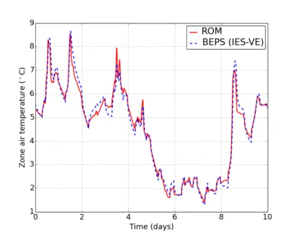
Fig. 3.3 Estimation of indoor temperature using IES-VE and reduced order model (ROM)
3.2
Formulation of Optimization Problem
3.2 Formulation of Optimization Problem 27
Unit Description
Tz ◦C Zone air temperature
Tsi ◦C Internal surface temperature
Tse ◦C External surface temperature
Tf ◦C Internal structures temperature
Ta ◦C Ambient temperature
Qs W Heat gains due to solar radiations
Qheat W Heat supplied by the heating system
Cp,z J/K Heat capacity of zone air
Cp,s J/K Heat capacity of structure
Cp,f J/K Heat capacity of internal mass
(UA)za W/K Heat transfer coefficient between zone air and ambient
(UA)z f W/K Heat transfer coefficient between zone air and internal mass
hi W/(m2K) Internal convective heat transfer coefficient
he W/(m2K) External convective heat transfer coefficient
As m2 Total surface area of external walls
ks W/mK Thermal conductivity of external wall
ts m Average thickness of external walls
Table 3.1 Description of model parameters
follow a prescribed target setpoint trajectory. In order to achieve this goal, a sequence of optimal control actions is needed which can maintain the zone temperature as close as possible to the target setpoints. This optimal control policy can be obtained by representing the considered objective function into a reference trajectory tracking optimization problem as following quadratic programming problem
min
u N−1
∑
i=0
3.3 Weather Forecast 28
subject to
xk+i+1=Adxk+i+Bduk+i+Edwk+i i=0,1, . . .N−1 (3.6a)
yk+i=Cxk+i i=0,1, . . .N−1 (3.6b)
umin≤uk+i≤umax i=0,1, . . .N−1 (3.6c)
∆umin≤uk+i−uk+i−1≤∆umax i=0,1, . . .N−1 (3.6d)
ymin−vk+i≤yk+i≤ymax+vk+i i=0,1, . . .N−1 (3.6e)
vk+i≥0 i=0,1, . . .N−1 (3.6f)
Here equation (3.5) represents the difference between actual temperature and the temperature calculated by the dynamical model for nextN time steps, whereN is the prediction horizon. In the above cost function, the system state of interest is only the zone temperatureTz, hence the value ofQcan be set toCTC. In equation (3.6 c),
umin andumaxrepresents the minimum and maximum possible values of heating
power that can be supplied to the building by the heating system. The equation (3.6 d) imposes the constraints on the rate of change of the control input for a safe operation of the heating system. Since the zone temperature may not be in the imposed constraint range always, hence the equations (3.6 e) and (3.6 f) establish
thesoft constraintson the indoor temperature which allows the zone temperature
to violate the constraint when necessary. ρ in the objective function represents
the penalty charged to controller from the violation of constraints. In this way the optimization routine seeks a compromise between minimizing the cost function and minimizing the constraint violations expressed byvi.
3.3
Weather Forecast
3.3 Weather Forecast 29
causal models. In time series models, weather data is modelled as a function of its past observed values and in causal model weather is modelled as some exogenous variable on which it depends causally. In the first class suggested, multiplicative au-toregressive models, dynamic linear or nonlinear models, threshold auau-toregressive models, and methods based on Kalman filtering are most used models. Some of the methods in second class are Box and Jenkins transfer functions, ARMAX models, op-timization techniques, nonparametric regression, structural models, artificial neural networks and curve-fitting procedures [19, 67].
In the following section, an efficient forecasting technique to predict weather data is used. The approach is suitable for real-time implementation of the control system.
3.3.1
Recursive ARIMA modelling
Auto Regressive Integrated Moving Average (ARIMA) models are quite popular in the field of time series forecasting. It has been used for forecasting in several disciplines like commodity price forecasting [45], electricity price forecasting [13, 12] and load forecasting [22, 10] etc.
In this chapter, a recursive ARIMA modelling approach is used to predict future ambient temperature and solar irradiance. The idea behind the technique is to use ARIMA models to make predictions over a rolling horizon, i.e. the parameters of estimated ARIMA model are updated at each time step. The basic idea of recursive ARIMA can be described in following steps
• Choose an appropriate ARIMA model to fit the given data
• Estimate the parameters of ARIMA model and forecast one step ahead value
• move the rolling horizon to next step and repeat above steps using updated real data
3.4 Forecasting using Recursive Seasonal ARIMA 30
is shown in figure 3.4 and 3.5. The length of the rolling horizon is considered to be 30 days. Therefore recursively at each time step, the data of last 30 days will be used to forecast and problem will be formulated again at next time step using the new available information. The mathematical details of the forecasting technique is described in next section.
3.4
Forecasting using Recursive Seasonal ARIMA
A time series is a sequence of data measured at regular points in time. In time series forecasting, a dynamical time series model is chosen to fit the time series data so that underlying dynamics of time series can be captured. Later, this model is used to make predictions about future values of time series.
Let us consider, a time series{Xt}is given wheret is the time index. The
predic-tion problem of time series can be defined as following
ˆ
Xt+k= f(Xt,Xt−1,Xt−2, . . .), k=1,2, . . . (3.7)
where Xˆt+k is the predicted value of Xt+k at time t. the value of k can be chosen
depending upon the problem. k=1refers to one-step ahead forecast.
First, some notations are introduced which are essential to discuss in order to analyse a time series.
• Differencing: Differencing transform a time series into a new difference series which consist of the difference between the series observation. The differencing-operator is denoted by∆dwhich representsdthorder differenced time series.
∆Xt=Xt−Xt−1
∆2Xt = (Xt−Xt−1)−(Xt−1−Xt−2)
Seasonal differencing∆Dcan also be applied to the time series at seasonal lag
3.5 Seasonal Arima Model 31
measured at monthly time steps then value of seasonality would be 12 and seasonal differencing is represented as following
∆12Xt=Xt−Xt−12
• Lag-operator: Another important notation in study of time series analysis is lag-operatorL. The lag operator shifts the time series by the specified lag as following
LiXt=Xt−i
So the first order difference of time series can be written using the lag-operator
L as (1−L)Xt =Xt−Xt−1. The seasonal differencing is represented by the
expression (1−LS)DXt, where Drefers to the order of seasonal differencing
with seasonal lagS.
3.5
Seasonal Arima Model
In lag operator polynomial notation, the seasonal ARIMA model can be specified by ARIMA(p,d,q)×(P,D,Q)s for time seriesXt with a seasonal periodSas following
φ(L)Φ(L)(1−L)d(1−LS)DXt =θ(L)Θ(L)εt (3.8)
whereφ(L) =1−φ1L−···−φpL,Φ(L) =1−Φ1L−···−ΦPL;θ(L) =1−θ1L−···−θqL
and Θ(L) = 1−Θ1L− ··· −ΘQL. εt is uncorrelated interference with zero mean.
The parametersp,P,qandQrepresents the degree of non-seasonal autoregressive, seasonal autoregressive, non-seasonal moving average and seasonal moving average polynomials. dandDrefers to the order of differencing.
3.5 Seasonal Arima Model 32
predicted and real data. The variance of prediction error data is notably low. The prediction error data time series looks nearly stationary.
0 10 20 30 40 50 60
Time [days] -5
0 5 10 15
Temperature [
°
C]
Ta
Fig. 3.4 Ambient temperature data used for recursive ARIMA forecasting
0 10 20 30 40 50 60
Time [days] 0
50 100 150 200 250 300 350 400 450 500
Solar irradiance [W/m
2]
Qs
Fig. 3.5 Solar irradiance data used for recursive ARIMA forecasting
3.5 Seasonal Arima Model 33
0 5 10 15 20 25 30
Time [days]
-2 0 2 4 6 8 10 12 14 16
Temperature [
°
C]
simulated temperature actual temperature
20.5 21 21.5 1
2 3
Fig. 3.6 Comparison between simulated temperature using recursive ARIMA and real temperature data
0 5 10 15 20 25 30
Time [days] -0.3
-0.2 -0.1 0 0.1 0.2 0.3 0.4
Prediction error [
°
C]
Fig. 3.7 Prediction error of temperature data with recursive ARIMA approach
3.6 Simulation Setup and Results 34
0 5 10 15 20 25 30
Time [days]
-50 0 50 100 150 200 250 300 350
Solar irradiance [W/m
2]
Simulated irradiance actual irradiance 4 5 6
0 20 40
Fig. 3.8 Comparison between simulated irradiance using recursive ARIMA and real irradiance data
0 5 10 15 20 25 30
Time [days] -150
-100 -50 0 50 100 150 200
Prediction error [W/m
2]
Fig. 3.9 Prediction error of irradiance data with recursive ARIMA approach
3.6
Simulation Setup and Results
de-3.6 Simulation Setup and Results 35
fines the range of indoor thermal environmental conditions acceptable to a majority of occupants. Time varying constraints for the indoor temperature are considered as following
yk,min=17◦C,yk,max=22◦C,yk,re f =19 k∈[6am−8 : 30am]ork∈[6pm−0.00am]
yk,min=14◦C,yk,max=18◦C,yk,re f =15 otherwise
(3.9)
yk,re f represents the tracking setpoint temperature during these intervals. The
maxi-mum heating or cooling power that heat-pump can provide is considered to be 10 kW and the maximum rate of change of control input is restricted at one-half of the maximum input power. The whole setup is simulated for 1 week.
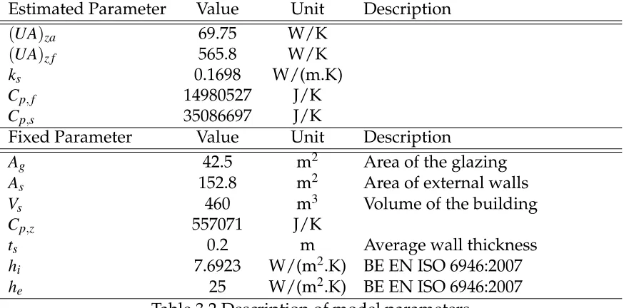
Estimated Parameter Value Unit Description
(UA)za 69.75 W/K
(UA)z f 565.8 W/K
ks 0.1698 W/(m.K)
Cp,f 14980527 J/K
Cp,s 35086697 J/K
Fixed Parameter Value Unit Description
Ag 42.5 m2 Area of the glazing
As 152.8 m2 Area of external walls
Vs 460 m3 Volume of the building
Cp,z 557071 J/K
ts 0.2 m Average wall thickness
hi 7.6923 W/(m2.K) BE EN ISO 6946:2007
[image:50.595.87.524.367.583.2]he 25 W/(m2.K) BE EN ISO 6946:2007
Table 3.2 Description of model parameters
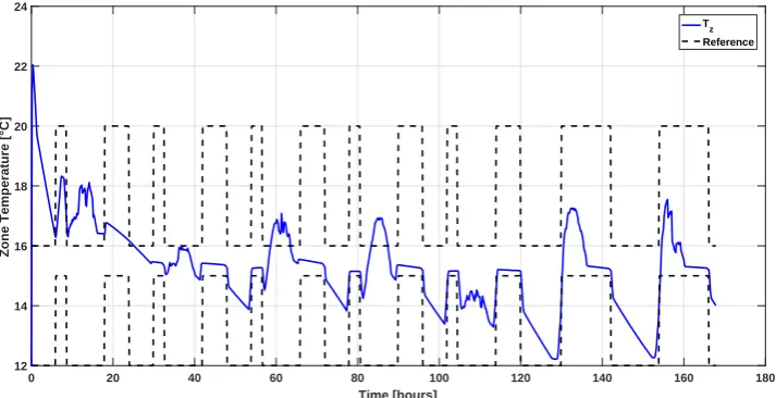
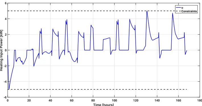
3.6 Simulation Setup and Results 36
is being cooled down. The heating input power is always maintained inside the constraints range.
0 20 40 60 80 100 120 140 160 180
Time [hours] 12
14 16 18 20 22
Zone Temperature [°C]
Tz
reference
Fig. 3.10 Zone temperature dynamics of the building
0 20 40 60 80 100 120 140 160 180
Time [hours]
-10 -8 -6 -4 -2 0 2 4 6 8 10
Power input [kW]
u Constraints
Fig. 3.11 Power input from HVAC to the building
3.7 Summary 37
3.7
Summary
Chapter 4
Model Predictive Control with
Cooperative Optimization Framework
In previous chapter, a base framework for model predictive control has been con-structed. Next, the MPC framework is extended to a group of buildings which are connected to shared heating systems (heat-pumps in this case) and propose a novel
cooperative optimization framework. Also, the advantages of the proposed framework
over the regularselfish optimization frameworkare investigated.
Different buildings differ in many ways such as their thermal inertia, envelope settings, occupant preferences and HVAC operation timings etc. The key idea of the framework is to exploit the added power capacity by sharing the heat-pump. For instance, if one building does not use the heating system at a particular time, then another building can use the additional buffer power capacity available to heat more flexibly.
4.1
Cooperative Optimization framework
4.1 Cooperative Optimization framework 39
further investigations on the energy performance of groups of building energy systems is needed.
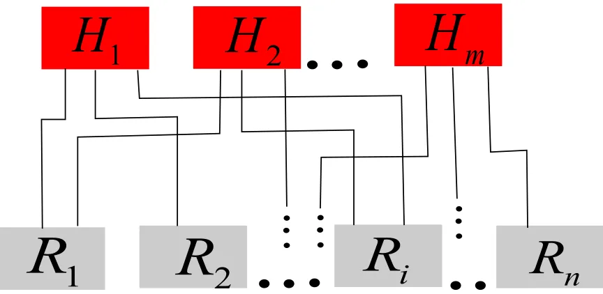
In this work, a group of buildings is considered which share a number of ground source heat-pumps. A prototype ofnbuildings andmheat pumps is developed as shown in figure 4.1. Rirepresents theith building andHjrefers to jth heat-pump.
1
H
2
H
m
H
1
R
2
R
R
i
[image:54.595.89.521.222.433.2]n
R
Fig. 4.1 Group ofnbuildings connected tomheat-pumps
Each heat pump may be connected to any number of buildings. The connectivity between the heat-pumps and buildings is represented mathematically by connectiv-ity matrixLwith dimensionn×m. If there is a connection betweenith building and
jth heat-pump then the value of the matrix entryL
i,j would be 1 and 0 otherwise.
The control influence matrix for the cooperative framework is given by
[Bs] = [B][L] (4.1)
where[B]is expressed as
[B] =h[B1] [B2] . . . [Bn]
i
4.1 Cooperative Optimization framework 40
and [Bi], i=1,2, . . . ,n denotes the control influence vector corresponding to the
buildingRiconnected with a heat pump.
The discrete time state-space model of the cooperative framework is represented as following
{xsk+1}= [As]{xsk}+ [Bs]{usk}+ [Es]{dsk}
{ysk}= [Cs]{xsk}
(4.3)
In equation (4.3),{xs},[As],{us},[Es],{ds},{ys}and[Cs]represent the augmented state
vector, state-transition matrix, control input vector, disturbance influence matrix, disturbance vector, output vector and the output influence matrix, respectively. These are given by
{xs}=
h
{x1}T {x2}T . . . {xn}T
iT
(4.4a)
[As] =Diag
h
[A1]T [A2]T . . . [An]T
iT
(4.4b)
{us}=
h
u1 u2 . . . um
iT
(4.4c)
[Es] =
[E1] [01] [01]. . . [01]
[01] [E2] [01]. . . [01]
..
. ... . .. ...
[01] . . . [En]
(4.4d)
{ds}=
h
{d1}T {d2}T . . . {dn}T
iT
(4.4e)
{ys}=
h
y1 y2 . . . yn
iT
(4.4f)
[Cs] =
[C1] [02] [02] . . . [02]
[02] [C1] [02] . . . [02]
..
. ... . .. . . . ...
4.2 Concept of MPC with Cooperative Optimization Framework 41
The matrices[01] and[02] are the matrices with all entries values to be zero with
dimensionns×randp×nsrespectively, wherens,randp, are the number of states,
number of disturbances and number of outputs for an individual building. The state vector, system matrix, disturbance influence matrix, disturbance vector, output vector and the output influence matrix for the buildingRj,j=1, . . . ,nare denoted by
{xj},[Aj],[Ej],{dj},{yj}and[Cj], respectively. The control input vector from each
heat pump is denoted by {uh},h=1, . . . ,m. Diagnotation is used to represent the
diagonal matrix with given entries.
4.2
Concept of MPC with Cooperative Optimization
Framework
In this section, the MPC approach is extended to cooperative optimization frame-work. If the buildings collaborate in sharing the heat pumps in energy distribution, then using the discrete-time linear state-space formulation to predict the future outputs of the system, an optimization problem can be formulated to minimize the total electricity consumption for operating all the heat-pumps while maintaining the indoor temperature of all the buildings in prescribed intervals. The constraints on the building dynamics and control input have to be satisfied here for all buildings. Hence, these conditions lead to a cooperative optimization problem in an MPC setting.
The objective of the control problem formulation is to minimize the total energy consumption. The MPC problem under cooperative optimization framework is formulated as following
min
xs,us,ysΦ=
N−1
∑
k=0
h m
∑
j=1∥
usjk∥∞+
n
∑
i=1 ρivik
i
4.3 Simulation Setup and results 42
subjected to
{xsk+1}= [As]{xsk}+ [Bs]{usk}+ [Es]{dsk}, k=0,1, . . .N−1 (4.6a)
{ysk}= [Cs]{xsk}, k=0,1, . . .N−1 (4.6b)
m
∑
i=1
uimin≤
∑
mi=1
uisk≤
∑
mi=1
uimax, k=0,1, . . .N−1 (4.6c)
m
∑
i=1
∆uimin≤
m
∑
i=1
∆uisk≤
m
∑
i=1
∆uimax, k=0,1, . . .N−1 (4.6d)
{yk,min} ≤ {ysk}+{vk}, k=0,1, . . .N−1 (4.6e)
{yk,max} ≥ {ysk} − {vk}, k=0,1, . . .N−1 (4.6f)
{vk} ≥ {0}, k=0,1, . . .N−1 (4.6g)
∥.∥∞ represent the uniform norm of the associated variable. In (4.6e), {yk,min}
and {yk,max} refer to the time-varying upper and lower limits of the temperature
comfort zone, respectively. {vk} is the vector of slack variables associated with
every building control system andρi is the respective penalty. In this way, if the
desired temperature demand cannot be achieved the optimization routine seeks a compromise between minimization of control input and the constraint violations expressed by {vk}. {umin} and {umax} is the vector of minimum and maximum
control input allowed. {∆umin}and{∆umax}impose constraints on the rate of change
of input.
4.3
Simulation Setup and results
For numerical simulation, three representative buildings are considered, namely a
small buildingwhich is low energy consuming residential building, alarge building
4.3 Simulation Setup and results 43
be identical. The value of the parameters of the buildings are set in appropriate proportion according to the size of the the building . All the buildings are subjected to the same outdoor weather conditions. The optimization framework is formulated in Matlab. The ambient temperatureTaand solar irradianceQs data is obtained from
global climate database provided by Meteonorm [3] with interpolation at every 10 minutes. These variables represent measured non-controllable disturbance inputs to the building. The historical weather data can be replaced by weather forecasts in a real-time implementation of the proposed algorithm. At each time step, the optimization problem is solved using the Mosek optimization [2] toolbox used with Matlab. The setup is simulated for 1 week period with a prediction horizon ofN = 144 (i.e. 24 hours). The maximum heat capacity of the heat-pump is considered 3.5 kW, 7.5 kW and 13.5 kW for small, large and office building respectively. Except the initial zone temperature, the initial system states are considered to be same for all the buildings.
The comfort zone range for small building is defined below as per ASHARAE comfort range for human occupancy [7]
yk,min=17◦C,yk,max=22◦C, k∈[6am−8 : 30am]ork∈[6pm−0.00am]
yk,min=14◦C,yk,max=18◦C, otherwise
(4.7)
For the larger building, the comfort temperature range is defined as
yk,min=16◦C,yk,max=21◦C, k∈[6am−8 : 30am]ork∈[6pm−0.00am]
yk,min=13◦C,yk,max=17◦C, otherwise
(4.8)
4.3 Simulation Setup and results 44
The constraints for the zone temperature of office building are imposed as fol-lows:
yk,min=15◦C,yk,max=20◦C, k∈[8am−6pm]
yk,min=12◦C,yk,max=16◦C, otherwise
(4.9)
4.3.1
Selfish Optimization
In the first scenario, the buildings do not share heat-pumps and each building is equipped with an individual heat-pump. This scenario is termed asselfish
optimiza-tion.
Selfish optimization with small and large building
Figure 4.2 shows the indoor temperature dynamics for the small building in the case when it is connected to one heat-pump which is not shared by the large building. Indoor temperature dynamics of the building depend upon the initial values of the system state. The temperature evolve in such a manner that the power consumption
0 20 40 60 80 100 120 140 160 180
Time [hours] 12
14 16 18 20 22
Zone Temperature [°C]
Tz
constraints
Fig. 4.2 Indoor temperature dynamics for small building with selfish optimization
4.3 Simulation Setup and results 45
0 20 40 60 80 100 120 140 160 180
Time [hours]
0 1 2 3 4 5 6
Heating Input Power [kW]
u Constraints
Fig. 4.3 Power consumption of heat-pump for small building with selfish optimiza-tion
time. In figure 4.3, the power consumption by the heat-pump in this case can be seen. The initial heating input power is high up to the maximum power capacity of the heat-pump because initial indoor temperature is lower than the minimum bound on the comfort zone. There is no power consumption during the time intervals when solar irradiance is high and yet the indoor temperature stay near the maximum bound on the comfort zone, even violates it slightly. In numerical simulation, last 48 hours correspond to weekend days for which the temperature constraints need to remain high to provide comfort to the occupant during the whole day. Consequently, there is a continuous power consumption by the heat-pump.
4.3 Simulation Setup and results 46
works throughout the simulation period. During the weekend days, the heat-pump compressor can be seen working persistently with maximum power consumption.
0 20 40 60 80 100 120 140 160 180
Time [hours] 11
12 13 14 15 16 17 18 19 20 21
Zone Temperature [°C]
Tz
constraints
Fig. 4.4 Indoor temperature dynamics for large building with selfish optimization
0 20 40 60 80 100 120 140 160 180
Time [hours] 0
1 2 3 4 5 6 7 8
Heating Input Power [kW]
u Constraints
4.3 Simulation Setup and results 47
Selfish optimization with office building
Figure 4.6 shows the indoor temperature variation in the office building. Zone temperature is maintained inside the defined comfort range. In figure 4.7, the power consumption profile of the heat-pump for this case can be seen. Since the initial indoor temperature is inside the comfort zone, the power consumption of the heat-pump is not very high as in the case of residential buildings. At the first day of weekend, the power consumption of the heat-pump drops drastically as the required comfort zone temperature is low during the weekend. Interestingly, the power consumption at the end of the simulation period is at a maximum so that the heat energy can be saved into the building envelop to satisfy comfort range requirements for the next day.
0 20 40 60 80 100 120 140 160 180
Time [hours] 11
12 13 14 15 16 17 18 19 20 21
Zone Temperature [°C]
Tz constraints
Fig. 4.6 Indoor temperature dynamics for office building with selfish optimization
4.3.2
Cooperative Optimization
4.3 Simulation Setup and results 48
0 20 40 60 80 100 120 140 160 180
Time [hours] 0
2 4 6 8 10 12 14
Heating Input Power [kW]
u Constraints
Fig. 4.7 Power consumption of heat-pump for office building with selfish optimiza-tion
the proposed approach. In the second case, one residential building and one office building are examined to account for different operation times of heating system.
Cooperative optimization with small and large building
4.3 Simulation Setup and results 49
the proposed framework can be seen in figure 4.10. The maximum peak load is curtailed by 14% with cooperative optimization framework in comparison to selfish optimization.
0 20 40 60 80 100 120 140 160 180
14 16 18 20 22
Zone Temperature [°C]
(a)
Tz constraints
0 20 40 60 80 100 120 140 160 180
Time [hours]
14 16 18 20
Zone Temperature [°C]
(b)
Tz
constraints
Fig. 4.8 (a) Indoor temperature dynamics for small building with cooperative op-timization, (b) Indoor temperature dynamics for large building with cooperative optimization
0 20 40 60 80 100 120 140 160 180
0 2 4 6
(a)
u
0 20 40 60 80 100 120 140 160 180
0 5 10
Power consumption [kW]
(b)
u
0 20 40 60 80 100 120 140 160 180
Time [hours] 0
5 10
(c)
u constraint
4.3 Simulation Setup and results 50
0 20 40 60 80 100 120 140 160 180
Time [hour] 3
4 5 6 7 8 9 10 11
Power consumption [kW]
selfish optimization cooperative optimization
Fig. 4.10 Total power consumption for both residential buildings with selfish and cooperative optimization
Cooperative optimization with office and residential building
Finally, the proposed cooperative optimization approach is implemented for the scenario when the small residential building and the office building share a single heat-pump. The main difference here from the previous scenario is the operation time of the heating systems for both of the buildings is different. The heating system in the office building is operated during office working hours. The residential building heating system functions almost in opposite hours to that of the office building as described in equations (4.7) and (4.9).
4.3 Simulation Setup and results 51
0 20 40 60 80 100 120 140 160 180
Time [hours]
14 16 18 20 22