Heterogeneous Auctions
PATRICIA ANTHONY and NICHOLAS R. JENNINGS University of Southampton
Due to the proliferation of online auctions, there is an increasing need to monitor and bid in multiple auctions in order to procure the best deal for the desired good. To this end, this paper reports on the development of a heuristic decision making framework that an autonomous agent can exploit to tackle the problem of bidding across multiple auctions with varying start and end times and with varying protocols (including English, Dutch and Vickrey). The framework is flex-ible, configurable, and enables the agent to adopt varying tactics and strategies that attempt to ensure that the desired item is delivered in a manner consistent with the user’s preferences. Given this large space of possibilities, we employ a genetic algorithm to search (offline) for effective strate-gies in common classes of environment. The stratestrate-gies that emerge from this evolution are then codified into the agent’s reasoning behaviour so that it can select the most appropriate strategy to employ in its prevailing circumstances. The proposed framework has been implemented in a simulated marketplace environment and its effectiveness has been empirically demonstrated.
Categories and Subject Descriptors: I.2.11 [Artificial Intelligence]: Distributed Artificial Intel-ligence—intelligent agents; K.4.4 [Computers and Society]: Electronic Commerce—distributed commercial transactions
General Terms: Algorithms, Design, Experimentation
Additional Key Words and Phrases: multiple auctions, bidding strategy, genetic algorithms
1. INTRODUCTION
Online auctions are a popular and effective medium for procuring goods and services in both business to business and business to consumer electronic com-merce [Bapna et al. 2001; He et al. 2003]. To date, there are more than 2500 auction houses that conduct business online.1Some of the well-known auction
1http://www.InternetAuctionList.com.
P. Anthony also wishes to acknowledge the funding of University Malaysia Sabah.
Author’s address: Intelligence, Agents, Multimedia Group, Department of Electronics and Com-puter Science, University of Southampton, Highfield, Southampton SO17 1BJ, United Kingdom; email:{pa99r, nrj}@ecs.soton.ac.uk.
Permission to make digital or hard copies of part or all of this work for personal or classroom use is granted without fee provided that copies are not made or distributed for profit or direct commercial advantage and that copies show this notice on the first page or initial screen of a display along with the full citation. Copyrights for components of this work owned by others than ACM must be honored. Abstracting with credit is permitted. To copy otherwise, to republish, to post on servers, to redistribute to lists, or to use any component of this work in other works requires prior specific permission and/or a fee. Permissions may be requested from Publications Dept., ACM, Inc., 1515 Broadway, New York, NY 10036 USA, fax:+1 (212) 869-0481, or [email protected].
C
houses include eBay,2 Amazon.com,3 Yahoo!Auction,4 Priceline,5 UBid6 and many others. These auction houses conduct many different types of auctions, but the more popular ones are English, Dutch, first-price sealed bid and second-price sealed bid (also known as Vickrey). In an English auction, the auctioneer begins with the lowest acceptable price and bidders are free to raise their bids successively until there are no more offers to raise the bid or until the end of the auction is reached if there is a time limit. The winning bidder is the one with the highest bid [McAfee and McMillan 1987]. A Dutch auction is the opposite of an English one in that the auctioneer starts with an initial high price, which is then lowered progressively until there is an offer from a bidder to claim the item. In the first-price sealed bid, each bidder submits their of-fer for the item without any knowledge of the others bids. The highest bidder gets the item and they pay a price equal to their bid. The Vickrey auction is similar to the first-price sealed bid auction, where the item is awarded to the highest bidder but they pay a price equal to the second highest bid [Vickrey 1961].
As the number of auction houses increases, consumers are faced with the problem of monitoring many auction sites, picking which auction to participate in, and making the right bid to ensure that they get the desired item under con-ditions that are consistent with their preferences. These processes of monitor-ing, selecting and making bids are both complex and time consuming. The task becomes even more complicated when there are different start and end times and when the auctions employ different protocols. For this reason, some online auctions provide bidding agents (proxy bidders) to assist consumers with these tasks.7In these systems, the consumer needs to supply their bidding agent with details of the item that they wish to purchase, as well as the maximum amount that they are willing to pay for it. The bidding agent then proceeds to bid in the auction and updates the consumer about the status of the auction from time to time until it terminates. While freeing the consumer to a certain extent, this type of facility typically has the problem of only being able to operate at a single auction site, or only operating with a single auction protocol. If the consumer wishes to participate in another auction, they need to wait until the auction is concluded to avoid getting multiple items. In addition, the auction site host could use information about the consumer to cheat them by manipulating the auction. This is possible in English auctions through shill bidding where bids are deliberately placed to drive up the price of an item [McAfee and McMillan 1992]. In this case, the consumer can be made to pay a price equal (or very close) to their maximum bid.
In view of these complexities, consumers tend to focus on a single auction of their choice. Unfortunately, winning in that auction does not necessarily mean
2http://www.ebay.com.
3http://www.amazon.com.
4http://auctions.shopping.yahoo.com.
5http://www.priceline.com. 6http://www.ubid.com.
that they get the best deal. They may have received a better price in another auction. The losers may also have had better luck in another auction as well. From the seller’s perspective, the lock in of bidders is also a disadvantage since those agents that value the good highly may not be amongst this set. This, in turn, restricts the expected revenue from the auction.
As a step toward the multiple auctions case, consumers can utilize the services of auction search engines (such as BidXS,8 AuctionWatch,9 and AuctionBeagle10). These allow the consumer to monitor multiple concurrent auctions, but they leave the actual bidding decision to the consumer. While this certainly increases the consumer’s knowledge of the global marketplace, it does not solve the problem of reducing the amount of time that has to be spent online. Moreover, deciding what amount to bid for an item requires an intelligent decision where the consumer needs to come up with a strategy to work out the bid value. In many cases, the outcome of this decision making is that the consumer is trapped with thewinner’s cursephenomenon where they pay more than the actual value of the item [Klemperer 1999].
To address these shortcomings, we believe it is necessary to develop an autonomous agent that can participate in multiple heterogeneous auctions, that is empowered with trading capabilities and that can make purchases au-tonomously. In more detail, the agent should monitor and collect information from the ongoing auctions, make decisions on behalf of the consumer and en-deavour to guarantee the delivery of the item. The agent must ensure that it never bids above the private valuation (the maximum amount that the con-sumer is willing to pay) and it tries to get the item in a manner that is consistent with the consumer’s preferences (e.g., at the earliest time, at the lowest price, or with maximum chance of succeeding).
To this end, this article reports on our work in developing such a bidding agent. The agent has a range of strategies that it can employ depending on the user’s aims and the environment in which the agent finds itself. Here we con-sider three different types of protocol: English, Dutch and Vickrey.11The strate-gies themselves are heuristic in nature because the multiple heterogeneous auction environment is very complex, dynamic and unpredictable, making it impossible to find an optimal strategy that can be used in practical contexts [Byde et al. 2002]. Moreover, our early investigations showed that the effective-ness of the strategies was heavily influenced by the nature of the environment [Anthony et al. 2001]. For this reason we decided to have different strategies for different circumstances. As the range of potential strategies is huge, we de-cided to use a genetic algorithm (GA) to search for effective strategies for each of the various environments that we identified [Anthony and Jennings 2002]. We chose this particular method because GAs have been known to perform well in areas where the space to be searched is large and not well understood
8http://www.bidxs.com.
9http://www.auctionwatch.com. 10http://www.auctionbeagle.com.
11The first-price sealed bid is not considered here because of its similarities (from a strategic point
[Mitchell 1996]. Having evolved the strategies, the agent adopts the one that is most appropriate to its prevailing context.
This paper advances the state of the art in the following ways. First, we develop a high level decision-making framework for an agent to bid across mul-tiple concurrent auctions of varying protocols with varying start and end times. This framework is heuristic in nature and uses tactics and strategies to vary the agent’s behavior so as to ensure a good fit with the user’s auction objectives. Second, we evolve a strategy that is effective in our multiple auction context. This strategy consists of multiple evolved sub-behaviors that are appropriate in different environmental settings and with different user objectives. This strat-egy is termed theintelligent bidding strategyin the remainder of this article. Third, we systematically evaluate the intelligent bidding strategy to highlight its operational characteristics in different scenarios.
The remainder of the article is structured in the following manner: In the next section, we describe our electronic marketplace scenario in which our al-gorithms are evaluated. Section 3 describes the fundamentals of the bidding algorithm and our initial evaluation of the various environmental factors that effect its performance. Section 4 describes the work on evolving strategies for particular classes of environments and the evaluation of the effectiveness of this method of approach. Section 5 describes and evaluates the intelligent bid-ding strategy. Section 6 discusses related work and finally, Section 7 presents our conclusions and further work.
2. THE ELECTRONIC MARKETPLACE
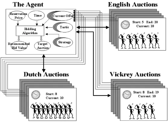
The simulated electronic marketplace consists of a number of auctions that run concurrently (see Figure 1).12There are three types of auctions running in the environment: English, Dutch and Vickrey. The English and Vickrey auctions have a finite start time and duration generated randomly from a uniform prob-ability distribution, the Dutch auction has a start time but no predetermined end time. The start and end times vary from one auction to another. At the start of each auction (irrespective of the type), a group of random bidders are generated to simulate other auction participants. These participants operate in a single auction and have the intention of buying the target item and pos-sessing certain behavior. They maintain information about the item they wish to purchase, their private valuation of the item (the maximum amount that they are willing to pay for the desired item), the starting bid value and their bid increment. These values are generated randomly from a standard proba-bility distribution. Their bidding behavior is determined based on the type of auction that they are participating in. In an English auction, they initiate bid-ding at their starting bid value; when making a counter offer, they add their
12The marketplace is a virtual simulation in that it is supposed to represent all the auctions that
Fig. 1. The Marketplace simulator.
bid increment to the current offer (provided the total is less than their private valuation), and they stop bidding when they acquire the item or when their private valuation is reached. In a Dutch auction, they wait until the offer value is equal to or less than their private valuation before making an offer. Finally, in a Vickrey auction, they bid at their private valuation. These strategies are all based on the dominant strategies of the respective one-shot single auctions [Sandholm 1999].
[image:5.612.173.451.116.325.2]The marketplace is flexible and can be configured to run any number of auctions and operate for any length of discrete time. We assume that all auctions in the marketplace are auctioning the item that the consumers are interested in. Our bidder agent is allowed to bid in any of the auctions and it aims to deliver the item to its consumer based on their preferences. The bidder agent is given a hard deadline by when it needs to obtain the item. The bidder agent utilizes the available information to make its bidding decision; this includes the consumer’s private valuation, the time it has left to acquire the item, the current offer of each individual auction, and its sets of tactics and strategies. The private valuation is derived from the item’s closing price distribution, observed from past auctions. The tactics and strategies are the main constituents that drive the agent’s behavior in making the bidding decision (these are described in Section 3). The output of the bidding decision is the auction the agent should bid in and the recommended bid value that it should bid in that auction. If the agent does not purchase the item by its deadline, it returns to the consumer for further instructions.
3. DESIGNING THE AGENT’S BIDDING STRATEGY
To ensure that our bidder agent operates effectively in the marketplace, it needs to possess a strategy to ensure that it obtains the item within the given time ac-cording to the consumer’s preferences. Here the bidding strategy for the agent is modelled on the idea of negotiation decision functions as proposed by Faratin et al. [1998]. The original model defined a range of strategies that an agent can employ to generate initial offers and counter offers in a two party negotiation. This model identifies the key constituents that drive an agent’s negotiation be-havior and defined a single tactic to deal with each of them. The agent’s overall behavior is then the amalgamation of these different facets, weighted by their relative importance to the user. Mapping this to an auction environment, the bidder agent needs to decide the new bid value based on the current offer price. The current offer can be treated as the offer and the new bid value can be treated as the counter offer. Negotiation is over when the auction terminates or when the bidder’s private valuation is reached (bidder walks out of the negotiation process).
First, we will present our notation. Lettbe the current universal time across all auctions, wheret ∈0, and0is a set of finite time intervals. Lettmaxbe the time by when the agent must obtain the good (i.e. 0≤t≤tmax), and letAbe the list of all the auctions that will be active before tmax. At any timet, there is a set of active auctionsL(t) whereL(t)⊂A. LetE(t),D(t), andV(t) be the set of active English, Dutch and Vickrey auctions, respectively, whereE(t)∩D(t)=φ,
D(t)∩V(t)=φ,E(t)∩V(t)=φ, andE(t)∪D(t)∪V(t)=L(t). Each auctioni∈ A, will have its own start time,σi, and its own end timeηi wherei ∈ E(t)∪V(t).
Letλbe the agent’s bid increment value, and prbe its private valuation for the
target item. LetItem NAbe a Boolean flag to indicate whether the target item has already been purchased by the agent. We assume that the value of pr is
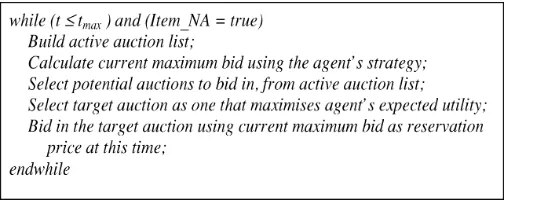
Fig. 2. Top-level algorithm for the bidding agent.
With these definitions in place, the algorithm for the bidding agent is sum-marized in Figure 2. Since each auction has a different start and end time, the bidder agent needs to build an active auction list to keep track of all the auc-tions that are currently active in the marketplace. We define an active auction as one that has started but not yet reached its end time. The agent identifies all the active auctions and gathers relevant information about them. It then calculates the maximum bid it is willing to make atthe current timeusing the agent’s strategy (described in Section 3.1). This current maximum bid, by defi-nition, will always be less than or equal to its private valuation. Based on the value of the current maximum bid, the agent selects the potential auctions in which it can bid and calculates what it should bid at this time in each such auction (described in Section 3.2). The auction and corresponding bid with the highest expected utility is selected from the potential auctions as the target auction. Finally, the agent bids in the target auction.
3.1 Calculating the Current Maximum Bid
At any given timet, the agent needs to determine its current maximum bid. This bid is defined as the maximum value that the agent is willing to offerat the
current moment in time. There are several factors that the agent needs to take
[image:7.612.186.453.118.225.2]The agent uses some combination of these constraints in order to determine its maximum bid value at the current moment in time. Our model is open in that if there was another aspect that the consumer wanted the agent to consider, then this could easily be added in as a new bidding constraint. Exactly which constraints are used in a given situation is determined by the consumers and their preferences. Thus, a consumer who wants to ensure it receives the item as quickly as possible would place the greatest weight on the time until deadline and the desperateness tactics, whereas a consumer who is looking to minimise the price paid would value the bargain tactic most highly.
More formally, letC be the set of considerations that the agent takes into account when formulating a bid and j represent the individual bidding con-straints, where j ∈ 1,. . .,|C|. Let1t denote the remaining time left for the agent to bid (i.e.,tmax−t) and1adenote the number of auctions left in the mar-ketplace. Letµdenote the agent’s desire for a bargain, whereµ∈[0, 1] (where 1 is actively looking for a bargain and 0 is not actively looking for a bargain), and εdenotes the agent’s level of desperateness for the item whereε ∈ [0, 1] (where 1 is very desperate and 0 is not desperate). For each of constraint j ∈C, there is a corresponding function fj(t) which suggests the value to bid based on
that constraint. These individual constraints are then combined using a func-tionFto produce the agent’s overall position. Examples forFinclude weighted average, max or min.
At a given time, the agent may consider any of the bidding constraints in-dividually or it may combine them depending on the situation (what the agent sees as being important at that point in time). In this work, if the agent com-bines multiple bidding constraints, it allocates weights to denote their relative importance. Thus, let wj(t) be the weight on constraint j at time t, where
∀j ∈C, 0≤wj(t)≤1, and P
j∈Cwj(t)=1.
The current maximum bid value for the agent at timet, is then calculated as
M(t)=Pj∈Cwj(t)fj(t). The agent uses a set of polynomial functions (drawn
from Faratin et al.’s [1998] negotiation functions) to calculate the bid value based on a single bidding constraint. Here this set of functions is referred to as the tactics. In the current implementation, the four tactics are remaining time, remaining auctions, desire for bargain and desperateness. The definition of each of these is given below.
3.1.1 The Remaining Time Tactic. This tactic determines the recom-mended bid value based on the amount of time remaining for the agent. Assume that the agent is bidding at time 0≤t≤tmax. The agent bids closer to
prastapproachestmax, and it eventually bids atprwhent=tmax. To calculate
the bid value at timet, the following expression is used:
frt=αrt(t)pr
whereαrt(t) is a polynomial function of the form:
αrt(t) = krt+(1−krt) µ
t tmax
¶1
β
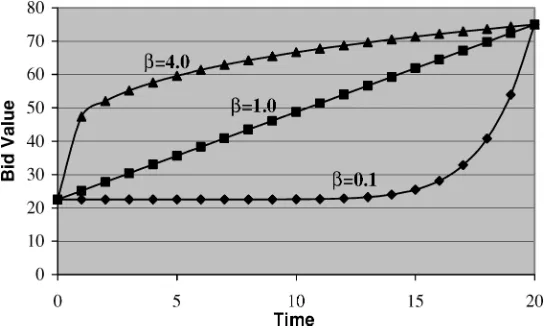
Fig. 3. Bid value for remaining time tactic withtmax=20 andpr=75.
krtis a constant that when multiplied by the size of the interval determines the
value of the starting bid of the agent in any auction. By varying the valueαrt(t),
a wide range of time-dependent functions can be defined from those that start bidding near pr quickly, to those that only bid near pr right at the end, to all
possibilities in between. The only conditions are that 0≤αrt(t)≤1,αrt(0)=krt, αrt(tmax)=1, and 0≤krt≤1.
Using the polynomial function defined in Eq. (1), different shapes of curve can be obtained by varying the values ofβ. This represents an infinite number of possible tactics, one for each value ofβ. In this tactic,β is drawn from<+, where 0.005≤β≤1000. Whenβ <1, the tactic maintains a low bid value until the deadline is almost reached, where this tactic concedes by suggesting the private valuation as the recommended bid value. The other extreme is when
β >1; the tactic starts with a bid value close to the private valuation and quickly reaches the reservation value long before the deadline is reached. By way of illustration, Figure 3 shows the different convexity degrees of the curves with
krt=0.30 andβ taking on the values 0.1, 1.0 and 4.0, respectively.
3.1.2 The Remaining Auctions Tactic. This tactic is broadly similar to the remaining time tactic; the agent bids closer to pr as the number of remaining
auctions approaches 0 (since it is running out of opportunities to purchase the desired item). Thus, frahas the same form as frtandαrais defined as follows:
αra=kra+(1−kra) µ
c(t)
|A|
¶1
β
Most of these terms are similar toαrt, the only difference being thatc(t) is the
list of auctions that have been completed between time 0 and timet.βis again drawn from<+, where 0.005≤β≤1000.
[image:9.612.176.449.118.282.2]it progresses fromt=0 totmax, but eventually bids its private valuation when
tmaxis reached. To determine the bid value for this tactic, the agent considers the minimum bid value for the target item across all the auctions in the mar-ketplace. At a given timet, newly started English auctions have low current bid values and Dutch auctions have very high current bid values. On the other hand, when auctions are terminating, English auctions typically have high current bid values and Dutch auctions have low current bid values. Vickrey auctions do not have any information on the bid values since bids are sealed and they are only opened at the end time. To deal with these points, the minimum bid value is calculated by taking into consideration the current bid value and the proportion of time left in the auction. These values are summed and averaged with respect to the number of active auctions at that time.
Let vi(t) be the current highest bid value in an auction i at timet, where
i∈L(t), andω(t) be the minimum bid value for the agent at timetwhere:
ω(t)= 1
|L(t)|
X
1≤i≤ |L(t)|
t−σi ηi−σi
vi(t) .
The bid value is then calculated using the expression:
fba=ω(t)+αba(t)(pr−ω(t))
whereαba(t) is defined as:
αba(t)=kba+(1−kba) µ
t tmax
¶1
β
. (2)
Assume thatαba(t) is similar to the polynomial function discussed in the first
two tactics, but this time, 0.1≤kba≤0.3, the minimum value ofβequals 0.005
and the maximum value ofβ equals 0.5. These values reflect the fact that an agent that is looking for a bargain should never bid with β >1 because this would inflate the agent’s bid well before the deadline. In contrast, an agent that is looking for a bargain (withβ < 1) maintains a low bid value until the deadline is almost reached where it will then suggest pr as the recommended
bid value. By conceding with a recommended bid value of pr, the agent tries to
ensure that it still successfully acquires the item even if it did not succeed in getting a bargain.
3.1.4 The Desperateness Tactic. This tactic is employed when the agent is desperate to get the item. The agent bids close to pr at t=0, and eventually
bids at pr whentmaxis reached. In this tactic, the agent utilizes the minimum bid value and the polynomial function of Eq. (2) but with a slight variation to the value ofβ, where 1.67≤β≤1000 and 0.7≤kde≤0.9. The values picked for
kdeare high since a desperate agent starts bidding at a value that is near pr.
3.2 Selecting Potential Auctions and the Target Auction
The agent selects potential auctions if and only if it is not holding the highest bid in an English auction or it has not placed a bid in a Dutch or a Vickrey auction. This is to ensure that the agent does not acquire more than one tar-get item. The agent selects the potential auctions by considering values for the current maximum bid for each active auction. In the English auctions, this is carried out by taking those auctions that are close to their end time, in which the current bid value when added to the bid increment is less than or equal to the current maximum bid. The agent’s new bid value is the current bid plus the bid increment. Only English auctions that are close to their end time are picked to maximise the agent’s chances of winning. If the agent currently holds a bid in an English auction that still has a long time to complete, it will not be able to participate in other auctions until it loses out to another bidder or until the auction terminates. There are several potential outcomes when an auction terminates; the agent loses out to another bidder; the agent’s bid value may be less than the private valuation (in which case there will be no winner); or the agent wins. If either of the first two situations occur, the agent loses out in that it wasted a lot of the time in one auction thus reducing its chances of par-ticipating in other auctions. The potential Dutch auctions in which the agent may bid are those with current bids that are less than the current maximum bid. Here, the agent’s new offer is the current bid for that particular Dutch auction. The potential Vickrey auctions in which the agent may bid are those that are terminating at the current time and the agent’s bid value is its current maximum bid value. The reason for this is because the timing of the bid does not affect the outcome of the auction, and so it is better to wait until the last minute [Byde et al. 2002] before placing a bid in a given Vickrey auction.
If there is only one auction in the potential auction list, that one is picked as the target auction. If there are multiple auctions, the agent calculates the ex-pected utility for each of them. By definition, the exex-pected utility is the product of the probability of the agent winning in that auction at the given bid value and the value of the agent’s utility function. The auction with the highest expected utility for the agent’s bid value is picked as the target auction. To calculate the agent’s probability of winning in an auction, we take into account the closing price distribution for all the auctions observed over time. In more detail, let
Pw
i (v) be the agent’s probability of winning in auctioniif it bids with the value
v. LetPc
i(p) be the probability of auctioniclosing at price p. The probability of
winning in an English or Vickrey auction is then:
Piw(v)=X
p>v
Pic(p)+ P
c i(v)
2
where
X
p<v
Pic(p)≤Piw(v)≤X
p≤v
Pic(p).
to the nature of the auction. In this situation, when the bid value is at pr, it is
almost certain that if our agent bids at that value it will win the auction unless there are collisions (when there is more than one bidder bidding for that item at a particular price). Letni be the number of bidders offering to buy the item
at the current offer price in Dutch auctioni, and letx be the number of Dutch auctions. The average number of collisions,θ, is then calculated as
θ=
P
ni
x .
Hence, the probability of winning in a Dutch auction is defined as Piw(v)=1θ. The expected utility for an auctioniwith a bid valuevis then calculated as:
ui(v)=Piw(v)Ui(v),
where
Ui(v)=1− µ
v pr
¶1
β
.
The β used here is the same as the one used in generating the polynomials for the tactics. The utility function for each potential auction is calculated by dividing the payoff amount with pr. The utility value is higher when the payoff
(pr−v) is high (value greater that 0), and it is lower when the payoff is low
(value close to or equal to 0).
3.3 Evaluating the Bidding Strategy
To evaluate the performance of our agent using the bidding algorithm described above, we undertook an empirical evaluation. We ran the experiments in an environment wheretmax=20. The total number of auctions running is between 20 and 30 and each auction has between 2 and 10 participants. The participants of the English and Vickrey auctions use the optimal (dominant) strategies to their respective one-shot auctions. For Dutch auctions, the participants wait until the offer value is just less than their pr before making an offer. In all
cases, the pr of these agents is drawn from the same probability distribution
as that of our bidding agent. Three control models are defined as a basis for comparisons. The first model (C1) simulates the behavior of a typical simple bidding agent that randomly joins one auction and stays there until its prhas
been reached or until the auction is over. In the second model (C2), the agent picks the auction that has the closest end time where the current bid is less than its pr, and stays there until the auction is over or until its pr is reached. The
third model (C3) is similar to C2 but the target auction is selected randomly. In both C2 and C3, if the item is not acquired, the process is repeated until the allocated time is over.
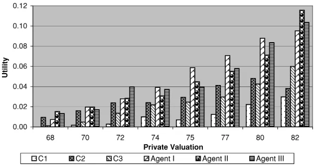
Experiments were conducted separately for different values of the user’s pri-vate valuation. Eight different experiments were conducted where each control model and bidding agent used pr values of 68, 70, 72, 74, 75, 77, 80 and 82.
Table I. Strategies for Bidding Agents
Pr Agent (krt,βrt) (kra,βra) (kba,βba) (kde,βde) (wrt,wra,wba,wde)
68
I (0.6, 500) (0.6, 500) (0.3, 0.5) (0.7, 500) (0.4, 0.2, 0.1, 0.3) II (0.8, 900) (0.8, 900) (0.8, 900) (0.4, 0.2, 0.0, 0.4)
III (0.9, 950) (0.9, 950) (0.5, 0.0, 0.0, 0.5)
70
I (0.6, 100) (0.6, 100) (0.3, 0.5) (0.7, 200) (0.4, 0.2, 0.1, 0.3)
II (0.7, 500) (0.8, 700) (0.5, 0.0, 0.0, 0.5)
II (0.8, 900) (0.9, 900) (0.5, 0.0, 0.0, 0.5)
72
I (0.6, 500) (0.7, 500) (0.5, 0.0, 0.0, 0.5)
II (0.6, 100) (0.6, 100) (0.3, 0.5) (0.7, 200) (0.25, 0.25, 0.25, 0.25) III (0.6, 100) (0.6, 100) (0.3, 0.5) (0.7, 200) (0.4, 0.2, 0.1, 0.3)
74
I (0.6, 150) (0.6, 150) (0.3, 0.5) (0.7, 150) (0.4, 0.2, 0.1, 0.3)
II (0.6, 200) (0.7, 200) (0.5, 0.0, 0.0, 0.5)
III (0.4, 500) (0.4, 500) (0.5, 0.0, 0.0, 0.5)
75
I (0.5, 100) (0.5, 100) (0.3, 0.5) (0.5, 100) (0.4, 0.2, 0.1, 0.3) II (0.6, 100) (0.6, 100) (0.3, 0.5) (0.7, 200) (0.4, 0.2, 0.1, 0.3)
III (0.6, 300) (0.7, 300) (0.5, 0.0, 0.0, 0.5)
77
I (0.6, 100) (0.6, 100) (0.3, 0.5) (0.7, 200) (0.25, 0.25, 0.25, 0.25)
II (0.5, 100) (0.6, 50) (0.5, 0.0, 0.0, 0.5)
III (0.5, 50) (0.5, 50) (0.5, 0.0, 0.0, 0.5)
80
I (0.3, 50) (0.3, 50) (0.2, 0.5) (0.3, 50) (0.25, 0.25, 0.25, 0.25)
II (0.2, 100) (0.2, 100) (0.5, 0.0, 0.0, 0.5)
III (0.2, 100) (0.3, 0.5) (0.2, 100) (0.4, 0.0, 0.2, 0.4)
82
I (0.1, 20) (1.0, 0.0, 0.0, 0.0)
II (0.1, 20) (0.3, 0.5) (0.3, 0.0, 0.7, 0.0)
III (0.1, 20) (0.1, 20) (0.2, 0.5) (0.1, 20) (0.25, 0.25, 0.25, 0.25)
different strategies that were employed by the bidding agents for each private valuation value.
As an example, Agent I withpr=68, values remaining time as the most
im-portant aspect (wrt=0.4), followed by the desperateness behavior (wde=0.3),
remaining auctions left (wra=0.2) and bargain (wba=0.1). It has a high
start-ing bid value and quickly reaches pr for the remaining time tactic and the
re-maining auctions left tactic. Its desire for a bargain is low (kba=0.3,βba=0.5)
but its level of desperateness is very high (kde=0.7,βde=500). Agent II with
pr=68 considers the remaining time left tactic and desperateness tactic as
equally important (wrt=0.4, wde=0.4). It considers the remaining auctions
left tactic as less important (wra=0.2) and is not looking for a bargain at
all (wba=0.0). It starts with a high bid value (krt=0.8, βrt=900, kra=0.8, βra=900,kde=0.8, andβde=900) and quickly reaches pr for all the three
tac-tics considered (this is why the column for the bargain tactic is left blank). The last agent for pr=68 (Agent III), considers the remaining time left
tac-tic and desperateness tactac-tic as very important (wrt=0.5, wde=0.5), and it is
not interested in the remaining auctions left tactic or the bargain tactic. For both tactics (krt=0.9,βrt=950,kde=0.9, andβde=950), the agent starts with
a high bid value and quickly reaches pr. These strategies are chosen because
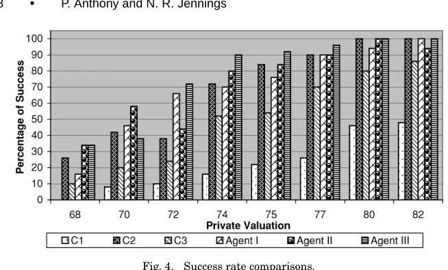
Fig. 4. Success rate comparisons.
For each pr, the three bidding agents with varying strategies and the three
control models were run for 100 times in the same environment, indepen-dently. Analysis of variance (ANOVA) was used to test the hypothesis about the differences between the success rate means (when running the experi-ment 50, 100, 150 and 200 times) [Cohen 1995]. The procedure revealed that for all the experiments, the differences between means were not significant (F3,8=0.027,p>0.05) and so the results obtained are statistically significant. Figure 4 shows the performance of the agents and the control models in terms of the success rate percentage. The success rate is the number of times, as a percentage, the agent is successful in obtaining the item. The first three bars represent the control models and the remaining three bars represent the three agents with three different bidding strategies. It can be seen that when pr is
low, the success rate is low. When pr is high, the agents have a better chance
of obtaining the desired item. At each pr point, the bidding agents performed
better than the control models. When the value of pr reaches 80 and 82, C2,
Agent I, Agent II, and Agent III achieved a 100% success rate, since the prior probability of winning in a single auction at this pr is very close to 1. In this
particular implementation, it is observed from the closing price distribution that the mean is 76 and the standard deviation is 5. This leads to the assumption that if the agent’spris 76, the probability of it winning in a single auction is 0.5.
The comparison for the average payoffs is shown in Figure 5. The average payoff is defined as P1≤n≤100(pr−vi/pr
n ), where vi is the winning bid value for
auctioni. The average payoff is calculated by deducting the agent’s bid value (the value at which it acquires the item) from the agent’s private valuation. This value is then divided by the agent’s private valuation, summed and averaged over the number of runs (in this case 100). Here, all three agents outperformed the control models for all prvalues. The payoffs obtained by the control models
are consistently lower than the bidding agents’ payoffs. It can also be seen that as pr increases, the payoffs that the bidding agents received also increased.
This indicates that the bidding agents actively looked for a bargain when their
[image:14.612.140.467.97.294.2]Fig. 5. Average payoff comparisons
The results of these experiments led to several conclusions. First, an agent that can bid effectively across multiple auctions is better than one that stays situated in a single auction. By being able to participate in multiple auctions, the agent is able to get a bargain (if it wishes to) by just changing the values of the bidding constraints. Secondly, the private valuation is one of the most im-portant factors that needs to be considered when determining the strategy that should be employed by the agent. This is important, for example, since an agent with a very lowprcannot look for a bargain and the agent should therefore
con-sider this when accepting the user’s preferences. The third observation is that the remaining time and remaining auctions tactics are the key determinants of successful behavior. Finally, the strategies to be used by the agent need to be dynamic, since not all strategies work well in all situations. Thus, a successful strategy in one situation may perform badly in another. However, it is possible to determine that certain classes of strategy are effective in environments that have particular characteristics. As an example, the agent strategy with val-ueskrt=0.60,βrt=100,kra=0.60,βra=100,kba=0.30,βba=0.50,kde=0.70, βde=200,wrt=0.40,wra=0.20,wba=0.10 andwde=0.30 was used three times
for pr values of 70, 72 and 75 respectively. It can be seen that it achieved the
highest success rate whenpris 72 but placed second highest when the private
valuation is at 70 and 75. Its average payoff is highest at pr=72 and pr=70
but it achieved second highest when pr=75. Here, we can conclude that this
strategy performs best atpr=72, but it does not necessarily perform well with
other values ofpr. However, this strategy did not perform well at pr=75 (even
though this value is higher than 72) because the allocated bidding time may be short and the number of auctions that it can participate in may be limited. In this case, the key defining characteristics of an environment were found to be the number of auctions that are active beforetmaxand the time the agent has to purchase the item (i.e.,tmax−tcurrent).
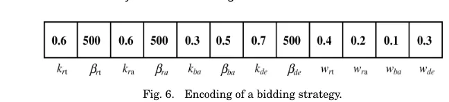
[image:15.612.154.472.116.285.2]Fig. 6. Encoding of a bidding strategy.
the next step is to determine which strategies should be used in which environ-ments. To this end, the next section discusses how we used GAs to address this problem.
4. EVOLVING BIDDING STRATEGIES
The performance of the bidding agent is heavily influenced by the strategy em-ployed, which, in turn, relates to the values ofkandβin the given tactics and the weights for each tactic when these are combined. The number of strate-gies that can be employed is infinite, so, therefore, is the search space. Thus, handcrafting strategies, as per the previous section, is not realistic in the long term. Thus a means of automating the process of finding successful strategies is necessary. For the reasons outlined previously, we decided to use GAs to search offline for the most successful strategies in the predefined environments. Based on the results of Section 3.3, the three key determinants for the strategy selec-tion are the remaining time left, the remaining aucselec-tions left and the private valuation. In this work, we defined four environments that take into accounts these determinants. The first one (STLA) is where there is a short bidding time (10≤tmax≤20) and a small number of active auctions in the marketplace (|L(t)| ≤10). The second environment (STMA) is where there is a short bidding time but the number of active auctions is large (11≤ |L(t)| ≤45). The third en-vironment (LTLA) is where the allocated bidding time is long (21≤tmax≤100) and where the number of active auctions is small. Finally, the last environment (LTMA) is where there is a long bidding time with many active auctions in the marketplace. Naturally, finer subdivisions are possible (see Section 5) but the focus here is demonstrating that strategies can be successfully evolved for broad classes of environments.
4.1 Encoding the Strategies
The individuals in the populations are the bidding agents and their genes con-sist of the parameters of the four different tactics and the relative weight for each tactic. Thus, the individuals are represented as an array of floating points values of:
(1) kandβ for the remaining time left tactic (2) kandβ for the remaining auctions left tactic (3) kandβ for the desire for a bargain tactic (4) kandβ for the desperateness tactic (5) the relative weights for the four tactics.
[image:16.612.132.456.103.177.2]column is treated as the gene. The first two columns indicate the agent’s values fork andβ for the remaining time left tactic, the next columns are the values forkandβ for the remaining three tactics and the last four columns represent the relative weight for each tactic.
4.2 Computing the Fitness Function
The fitness function measures how well the individual performs against the others. Designing the fitness function is one of the key facets of GAs and so here we consider three plausible alternatives. These are the individual success rate in obtaining the item (Fitness Equation 1) and two variations based on the average utility. In the first case (Fitness Equation 2), the agent gets a util-ity of 0 if it fails to obtain the item. If it is successful, the utilutil-ity of winning in an auctioni is computed as Ui(v)=(prp−rv)+c, wherev is the winning bid
andcis an arbitrary constant ranging from 0.001 to 0.005 to ensure that the agent receives some value when the winning bid is equivalent to its private valuation. The final utility function (Fitness Equation 3) is similar to Fitness Equation 2 but the individual is penalised if it fails to get the item. In this case the penalty incurred ranges from 0.01 to 0.05. These values were chosen to analyse how the population evolves with varying degrees of penalty. Intu-itively, Fitness Equation 1 should be used if delivery of the item is of utmost important, Fitness Equation 2 should be used if the agent is looking for a bar-gain and Fitness Equation 3 should be used when delivery of the item and looking for a bargain are equally important. The fitness score is then computed by taking the average utility from a total of 2000 runs. It is necessary to run these 2000 times to decrease the estimated standard error of the mean to a minimal level (when the number of runs is 500, the standard error of the mean is 5.0458, but this figure is significantly reduced to 1.1559 when the number of runs is increased to 2000). Analysis of Variance (ANOVA) was also used to test hypothesis about the differences between the fitness score means collected for the different number of runs. The null hypothesis of equal means was rejected because the procedure revealed that for all the experiments, the differences between means were significant (F4,245=675.182, p<0.05) and so the results are statistically significant.
4.3 Searching for Successful Strategies
The algorithm for searching for acceptable strategies in a given environment is shown in Figure 7 and is elaborated upon in the remainder of this subsection.
Fig. 7. The strategy searching genetic algorithm.
4.3.2 The Selection Process. The purpose of the selection process is to en-sure that the fitter individuals are chosen to populate the next generation in the hope that their offspring will in turn have higher fitness [Beasley et al. 1993a]. “Elitism” is used here to force the GAs to retain some number of the best individuals at each generation [Mitchell 1996], since such individuals can be lost if they are not chosen to reproduce or if they are destroyed by crossover and mutation. Ten percent of the best individuals are copied to the new pop-ulation to ensure that a significant proportion of the fitter individuals make it to the next generation. The remaining ninety percent of the individuals in the population are then chosen using Tournament Selection [Blickle and Thiele 1995b]. The selection is performed by choosing some numberϕ from the pop-ulation and the best individual in this group is copied into the intermediate population (which is referred to as the mating pool). This process is repeated for 90% of N times. This selection technique is known to work well since it allows a diverse range of fit agents to populate the mating pool [Blickle and Thiele 1995a]. Once the mating pool is created, the individual with highest fit-ness is selected and moved to the new generation. The remaining individuals go through the process of crossover and mutation before making it to the new population. The new population includes a group of the fittest individual and the offspring generated from the reproduction process.
4.3.3 The Crossover Process. This process exchanges the genes between individual agents. Two individuals are randomly selected from the mating pool with crossover probability of pc=0.6, and the crossover point (c) is equal to 2.
[image:18.612.180.415.105.269.2]The new values are then generated between the minimum and maximum range.
4.3.4 The Mutation Process. Mutation allows the population to explore the search space but at a slower rate. In this work, individuals from the population are selected to mutate with a probability ofpm=0.02. The gene from the chosen
individual is picked randomly and a small value (0.05) is added or subtracted, depending on the range limitation for that particular gene. The mutation pro-cess is only applied to the values ofkandβfor each tactic. The weights are not considered here because adding a small value to the weight requires a renor-malization and will have very little effect on the agent’s online behavior.
4.3.5 The Stopping Criterion. The process terminates when the population converges. This is a condition where the population evolves over successive generations such that the fitness of the best and the average individual in each generation increase toward a global optimum [Beasley et al. 1993a]. The global optimum is defined as the highest peak in the search space [Mitchell 1996]. In this case, the population always converges before 50 iterations (typically, the value lies between 24 and 40).
4.4 Evaluating the Evolved Strategies
The aim of these experiments is to show that GAs can be used to evolve strate-gies that are effective in particular environments. To this end, the GAs are run in four different environments (in which the agent’spris set to 75). For each
en-vironment, we use the three different fitness functions described in Section 4.2. Apart from determining the strategies that work well in a given context, these experiments also aim to evaluate the strategies in terms of their success rate and the average payoff in a similar manner to the experimental evaluation con-ducted in Section 3.3. However, the key difference is that, here, the performance of the agents is evaluated based on an environment that has a particular set of characteristics. The performance of the evolved strategies is then compared with that of a control modelC.C’s strategy is to bid in the auction that has the closest end time where the current bid is less than its pr. This model was
chosen because it performed well in the previous experiment as reported in Section 3.3 (in fact, this is C2). We also ran another set of experiments in the subenvironment of short time less auctions (STLA) in which the value of pr is
varied between a low value of 68, a medium value of 76 and a high value of 82. The purpose of this is to determine how the strategies evolve when varying pr.
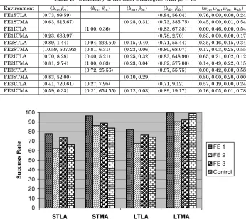
Turning to the first set of experiments (summarized in Table II). These re-sults show the best strategies that have evolved for the different classes of environment. Each row contains the resulting strategies for each environment using Fitness Equations 1, 2 and 3.13The values for the tactics are expressed as a pair ofk andβ and the weights for the bidding constraints are expressed as (wrt,wra,wba,wde). When a particular tactic is not present in the evolved
13FE1 indicates Fitness Equation 1, FE2 indicates Fitness Equation 2 and FE3 indicates Fitness
Table II. Summary of the Best Strategies withpr=75
Environment (krt,βrt) (kra,βra) (kba,βba) (kde,βde) (wrt,wra,wba,wde)
FE1STLA (0.73, 99.59) (0.84, 56.04) (0.76, 0.00, 0.00, 0.24) FE1STMA (0.63, 515.67) (0.28, 0.31) (0.73, 385.75) (0.45, 0.00, 0.01, 0.54) FE1LTLA (1.00, 0.36) (0.83, 67.38) (0.00, 0.46, 0.00, 0.54) FE1LTMA (0.23, 683.97) (0.78, 2.70) (0.83, 0.00, 0.00, 0.17) FE2STLA (0.89, 1.44) (0.94, 233.50) (0.15, 0.40) (0.71, 55.44) (0.35, 0.16, 0.15, 0.34) FE2STMA (10.59, 507.92) (0.81, 6.31) (0.23, 0.06) (0.80, 68.07) (0.17, 0.03, 0.25, 0.55) FE2LTLA (0.70, 8.28) (0.40, 5.21) (0.25, 0.32) (0.83, 648.90) (0.65, 0.21, 0.02, 0.12) FE2LTMA (0.81, 9.74) (1.00, 0.83) (0.23, 0.04) (0.82, 575.00) (0.14, 0.49, 0.22, 0.15) FE3STLA (0.72, 25.56) (0.87, 55.75) (0.00, 0.42, 0.00, 0.58) FE3STMA (0.83, 52.00) (0.10, 0.29) (0.80, 0.00, 0.20, 0.00) FE3LTLA (0.41, 720.61) (0.27, 7.95) (0.71, 9.12) (0.57, 0.19, 0.00, 0.24) FE3LTMA (0.59, 0.33) (0.21, 654.55) (0.12, 0.03) (0.89, 19.17) (0.16, 0.05, 0.01, 0.78)
Fig. 8. Agent’s performance in terms of success rate.
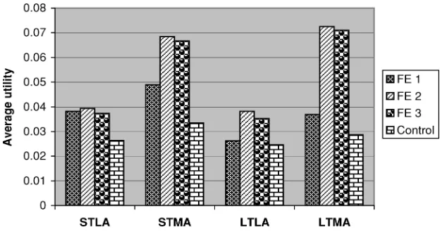
strategy, the cell corresponding to it is blank. The utilization of the differ-ent fitness functions reflects the varying behavior that the agdiffer-ent can employ in a given situation. It can be observed that the agents that utilised Fitness Equation 1 (where delivery is of utmost important) did indeed score a higher percentage in terms of success rate than the agents that used the other two fitness functions (see Figure 8) and the control modelC, for all environments. Agents that used Fitness Equation 2 achieved the highest utility in all the en-vironments (see Figure 9), whereas agents that used Fitness Equation 3 strike a balance between a high success rate and a high payoff. These results are very much as expected (see Section 4.2).
In the STLA environment based on Fitness Equation 1, the dominant strat-egy that emerged is the combination of the remaining time and the desper-ateness tactics (wrt=0.76,wde=0.24). In this particular situation, the agent’s
initial bids in both tactics are high and the agent quickly reaches its pr
(krt=0.73,βrt=99.59,kde=0.84,βde=56.04). This behavior is rational since an
Fig. 9. Agent’s performance in terms of average utility.
one that utilises all the tactics, but that places more importance on the remain-ing time and desperateness tactics. This is because the agent that is lookremain-ing for a high payoff should consider the bargain tactic as one of the tactics to ensure a higher payoff. The strategy that emerged based on Fitness Equation 3 is one that considers the remaining auctions left and the desperateness tactics where the agent’s initial bid is high and quickly reachespr. This strategy is similar to
the one that emerged from Fitness Equation 1, but the rate at which it reaches
pr is slower. The reason for this is that an agent that is looking to maximize
the payoff whilst ensuring delivery of the item needs to maintain a balance between a low bid price and the rate at which it reachespr.
In the STMA environment, an effective strategy should consider the remain-ing time and desperateness tactics highly since the allocated biddremain-ing time is limited (as per STLA). This is true when delivery of the item is important (as reflected in Fitness Equation 1’s result), but also when payoff (refer to result of Fitness Equation 2) is the main consideration (here the agent combines all the tactics but heavier weights are placed on the desperateness and bargain tactics). This situation differs from STLA because here, the agent can afford to spend some time looking for a bargain since the number of active auctions is large. The dominant strategy that emerged based on Fitness Equation 3 is surprising because it combines the remaining time and the bargain tactics, instead of deploying a more aggressive behavior of combining the remain-ing time, desperateness and the bargain tactics. In this case, the strategy is aware of the large number of active auctions so it tries to get a higher pay-off, but at the same time it takes into account the length of time it has left to bid.
[image:21.612.155.472.116.281.2]Table III. Strategies for STLA with Varying Private Valuations
pr (krt,βrt) (kra,βra) (kba,βba) (kde,βde) (wrt,wra,wba,wde)
68 (0.64, 5.44) (0.57, 79.37) (0.11, 0.15) (0.75, 466.24) (0.12, 0.00, 0.00, 0.88) 76 (0.05, 0.99) (0.58, 508.59) (0.23, 0.08) (0.90, 86.53) (0.00, 0.17, 0.00, 0.83) 82 (0.07, 97.11) (0.06, 12.37) (0.17, 0.46) (0.75, 4.74) (0.36, 0.35, 0.18, 0.11)
Fig. 10. Agent’s performance with varying private valuations.
based on Fitness Equation 3 considers the remaining time, remaining auctions and desperateness tactics. Bargain is not considered here, since the number of active auctions in the marketplace is small (as per STLA).
All the strategies that evolved in the LTMA environment, for all fitness func-tions, achieved more than 90% success rate, but they differ in terms of payoff. The reason for this high success is due to the long bidding time, as well as the large number of active auctions that agents can participate in. Hence, the agent has many chances of winning. In this particular situation, the main considera-tion is the payoff. As can be seen, the strategies that utilised Fitness Equaconsidera-tion 2 and 3 generate higher payoffs when compared to the strategy that evolved based on Fitness Equation 1 and the control modelC. The reason for this is that both
Cand Fitness Equation 1 consider delivery as the most important criteria and payoff is not taken into account.
Turning now to the second class of experiments. Table III shows the strate-gies that evolved in the STLA environment based on Fitness Equation 3. Fitness Equation 3 is used here since it offers a reasonably high success and payoff. In this context, Figure 10 shows that the success rate and the payoff increase when
pr increases. The high payoff that the agent receives when using the strategy
evolved with prindicates that the agent actively tries to look for bargain when
private valuation is high (pr=82). In contrast, when the private valuation is low
(pr=68), the agent evolves a strategy that combines the remaining time and
the desperateness tactics to take advantage of the limited time, limited num-ber of active auctions and limitedpr. The strategy that emerged withpr=76 is
similar to the one that evolved with pr=68, but this time, it considers the
valuation, the agent has a better chance of obtaining the item, enabling it to switch to a strategy that focuses on the desperateness tactic and the remaining auctions left tactic. When pr is high, the strategy that emerged considers all
tactics as expected. These results led us to conclude that evolving the strategies for finer subdivisions (e.g., by further partitioning the STLA environment into more private valuation divisions) will better tune the agent’s bidding strategy and result in a more superior performance.
In summary, several conclusions can be drawn from these results. First, GAs can be used to evolve strategies that are successful in particular environments (in all cases, performance is superior to the control model). Second, when se-lecting a strategy to bid in the multiple auctions environment, the agent needs to determine the current environment’s type, as well as the user’s preferences. Depending on these two, it can then decide which strategy to deploy. The re-sult presented in Figure 10 shows that as the private valuation increases, the success rate increases, therefore allowing the strategy to deploy a bargaining behavior to generate a higher payoff. Finally, the results also indicate that the categories of environment for which the strategies need to be evolved can be further subdivided into finer divisions so that the agent can better tune its bidding strategy to its prevailing circumstances.
5. THE INTELLIGENT BIDDING STRATEGY
Having shown that GAs can effectively evolve strategies for different environ-ments, the final step is to combine this knowledge into a single intelligent bid-ding agent. This agent has at its disposal knowledge about which strategies are effective in which environments and, assuming it can assess the environment accurately, it simply has to deploy the appropriate strategy.
Table IV. The Environments
STLA STLA STLA
STMA STMA STMA
FE1 MTLA FE1 MTLA FE1 MTLA
MTMA MTMA MTMA
LTLA LTLA LTLA
LTMA LTMA LTMA
STLA STLA STLA
STMA STMA STMA
RP1 FE2 MTLA RP2 FE2 MTLA RP3 FE2 MTLA
MTMA MTMA MTMA
LTLA LTLA LTLA
LTMA LTMA LTMA
STLA STLA STLA
STMA STMA STMA
FE3 MTLA FE3 MTLA FE3 MTLA
MTMA MTMA MTMA
LTLA LTLA LTLA
LTMA LTMA LTMA
RP1: Low Private Valuation STLA: Short Time Less Auctions RP2: Medium Private Valuation STMA: Short Time Many Auctions RP3: High Private Valuation MTLA: Medium Time Less Auctions FE1: Fitness Equation I MTMA: Medium Time Many Auctions FE2: Fitness Equation II LTLA: Long Time Less Auctions FE3: Fitness Equation III LTMA: Long Time Many Auctions
The categorization of the private valuation is made based on the auction closing price distribution (as per Section 3.3, the closing price mean is 76 and the standard deviation is 5). Fifty percent of the auctions should be won by bidders with medium private valuations, 25% by bidders with low private val-uations and the remaining 25% by the bidders with high private valuation. In real market settings, the price of each desired item will naturally vary depend-ing on the type of the item itself (e.g., a diamond rdepend-ing usually costs more than a book). However, the value of a given item can be directly mapped to the reser-vation price categorisation merely by obtaining the mean price of the item. This can be achieved using comparison price data from sites such as PriceSCAN,14 DealTime,15and BottomDollar.16From this, the agent can calculate the mean price of a given item and regenerate price ranges for the low, medium and high private valuations. The subdivisions of the short time, medium time, long time, less auctions and many auctions can also be carried out in a similar manner.
We then used the search algorithm defined in Section 4.3 to evolve the best strategy for each environment. Thus, the agent gets the user’s private valuation, the item to be purchased, when it is required and the intention of the user (either looking for a bargain, desperate or some combination of the two). With this knowledge, the agent enters the marketplace and determines the number of active auctions in which it can participate within the given time constraint. Based on this combination of information, the agent determines which strategy
14http://www.pricescan.com/. 15http://www1.dealtime.com/.
to use in each auction round. This decision is captured in a rule base that maps the prevailing context to the strategy that has been evolved for that situation (see Table V). Upon selection of the appropriate strategy the agent proceeds as defined in Figure 2.
5.1 Experimental Evaluation
The hypothesis that we seek to evaluate in this section is that our intelligent bidding strategy performs effectively in a wide range of bidding contexts. Here, the performance of the agent is measured in terms of success rate and aver-age utility (as defined in Section 4.4). As our control models, we use an aver-agent (C1) that has a single fixed strategy based on the user’s behavior and an agent (C2) that possesses a random behavior. In particular, we picked the strategy that was evolved for the environments RP2FE1MTMA, RP2FE2MTMA and RP2FE3MTMA (as discussed in Section 4.4)17forC1. Thus,C1 has three dif-ferent strategies; when a user is interested in a bargain,C1 selects the strategy that was evolved for RP2FE2MTMA, when a user is desperate for the item,C1 employs the strategy that was evolved for RP2FE1MTMA and when a user is looking for a combination of both, it utilises the strategy evolved based on RP2FE3MTMA. In particular, Table VI shows the values of the respectivek,β, and the weights for each bidding constraint employed byC1. ControlC2, on the other hand, is an agent that utilises a strategy in line with the user’s preference that is randomly picked (for each run) from those listed in Table V. Thus, if a user is interested in a bargain, the agent randomly selects any of the 18 strate-gies in FE2. When a user is desperate for the item, the agent selects randomly from the strategies in FE1. Finally, when a user is looking for a combination of both, the agent selects the strategies in FE3 randomly. It was decided to use three strategies for the control models, rather than a single strategy, so that we could measure the performance of the agents in terms of the individual user’s preferences. At any point in time, our intelligent agent will always possess one behavior (looking for a bargain, desperate or some combination of these two). Obviously, if its behavior is one that is interested in a bargain, the average utility should be high, but the success rate may be low. The converse of this is when our intelligent agent possesses desperate behavior; the success rate should go up, but the average utility may go down. Thus, to compare like with like, we consider the control model as similarly having the strategy that seeks to maximize the desired user behavior.
The experimental set up is broadly as described in Section 3.3. In particu-lar, the agent and the control model were run 1000 times in the marketplace. ANOVA was used to test the hypothesis about the differences of the success rate means (when running the experiment 200, 400, 600, 800 and 1000 times) and the procedure revealed that for all experiments, the differences between means were not significant (F4,15)=0.134, p>0.05. Thus, the results obtained are statistically significant. The user’s requirement was randomly allocated;
17We chose these environments because the average time to procure the good in the marketplace is
Table V. Strategies for the Intelligent Agent
Behavior (krt,βrt) (kra,βra) (kba,βba) (kde,βde) (wrt,wra,wba,wde)
Table VI. Strategies for the Control Model C1
Behavior (krt,βrt) (kra,βra) (kba,βba) (kde,βde) (wrt,wra,wba,wde)
RP2FE1MTMA (0.89, 32.56) (1.00, 0.09) (0.14, 0.21) (0.82, 3.57) (0.95, 0.05, 0.00, 0.00) RP2FE2MTMA (0.83, 2.41) (0.83, 78.85) (0.17, 0.12) (0.76, 648.30) (0.21, 0.60, 0.07, 0.12) RP2FE3MTMA (0.92, 963.71) (0.16, 0.48) (0.15, 0.13) (0.84, 57.56) (0.00, 0.08, 0.00, 0.92)
Fig. 11. Success rate comparisons.
the private valuation ranges from 70 to 82 and the time allocated ranges from 10 to 100.18 The user’s intention is also generated randomly. The number of auctions running in the marketplace is between 2 and 60 and, as before, there are between 2 and 10 participants in each such auction.
The performance of the intelligent agent and the control model in terms of success rate is shown in Figure 11. The experiment is divided into four groups. The first three groups show the detailed performance of the agent and the control models based on a single behavior (desperateness, bargain, and both) and the last group shows the overall performance when all three behaviors are considered. It can be seen that our intelligent agent achieved a higher success rate for all the individual user behaviors and for the overall behavior. In desperateness mode, the intelligent agent achieved a 7% higher success rate thanC1 and a 14% higher success rate thanC2. This shows that by having the ability to change the strategy in accordance with the user’s preference and the environment it is situated in, our agent can maximize its chances of succeeding. This is different fromC1, in which a fixed strategy is used and where the agent views the environment and user’s preferences as static. In this case,C1 was only successful in the environment for which it was evolved (RP2FE1MTMA).
C2 achieves a lower success rate when compared to our intelligent agent and
C1. Since the strategy selection in C2 is random, the strategy selected may not be suitable for the environment that the agent finds itself in. The situation
18This is slightly different from the two previous experiments in that the private valuation and the
Fig. 12. Average utility comparisons.
is similar when our intelligent agent is in bargain mode. It achieved a higher success rate when compared to the two control models. When both bargain and desperation are considered, our intelligent agent also achieved a higher success rate than the control models. In both cases,C1’s performance is lower because its fixed strategy is inappropriate.C1 starts bidding at a low value and slowly reaches its private valuation. Such a strategy is simply not effective in environments where there is a short bidding time, low private valuations or few active auctions in the marketplace. C2 picks its strategy without taking into account the nature of its environment, resulting in a lower performance when compared to bothC1 and our intelligent agent. When all these behaviors are combined, our intelligent agent achieved 12% higher success rate than the control models.
Figure 12 shows the average utility obtained by the intelligent bidding agent and the control models. It can be seen that our agent performed well compared to the control model and it achieved a high average utility in all cases. However, in the desperateness mode, our agent’s average utility surpassed the control models’ average utility by only a small value (0.00077 more thanC1 and 0.00175 more thanC2). The reason for this can be attributed to the strategies used in
C1 andC2. The former uses a fixed strategy that enables it to perform well in the RP2FE1MTMA environment and possibly the RP3 environments. This is because with a higher private valuation,C1 has more chances of obtaining the item irrespective of its strategy. In this case, when it wins the auction, it will definitely obtain a high payoff resulting in a high average utility. In the latter case, when the private valuation falls into the RP3 category, the strategy picked yields a higher payoff than the others and this also results in a higher average utility. This is not the case for our intelligent agent because it uses a strategy that is evolved based on the current environment where it is not interested in obtaining a higher utility (rather it is interested in the delivery of the required item).
[image:28.612.143.462.99.282.2]