Temperature effects on the activity coefficient of the bicarbonate ion

Thesis by

Fernando Cadena Cepeda

In Partial Fulfillment of the Requirements for the Degree of

Doctor of Philosophy

California Institute of Technology Pasadena, California

1977

ACKNOWLEDGMENTS

I would like to acknowledge my fiancee, Stephanie Smith, and thank her for her love and moral encouragement during my studies at Caltech. I would also like to thank her for her excellent typing of this thesis.

I am especially grateful for my advisor, Dr. James J. Morgan, for his interest and guidance in the preparation of this work.

I would also like to thank the Mexican Commission of Science and Technology, CONACYT, for financing my studies while in the United States.

I extend my deep appreciation to my parents, Mr. and Mrs. Raul Cadena, for their constant interest in my well being.

I am appreciative for the faculty of Environmental Engineering at Caltech for their excellent teaching.

I extend my grateful appreciation to my friends at Lake Avenue Congregational Church for their prayers and moral support.

ABSTRACT

Natural waters may be chemically studied as mixed electrolyte solutions. Some important equilibrium properties of natural waters are intimately related to the activity-concentration ratios (i.e., activity coefficients) of the ions in solution. An Ion Interaction Model, which is based on Pitzer's (1973) thermodynamic model, is proposed in this dissertation. The proposed model is capable of describing the activity coefficient of ions in mixed electrolyte solutions. The effects of

temperature on the equilibrium conditions of natural waters and on the activity coefficients of the ions in solution, may be predicted by means of the Ion Interaction Model presented in this work.

The bicarbonate ion, _{Hco3 -,} is commonly found in natural waters. This anion plays an important role in the chemical and thermodynamic properties of water bodies. Such properties are usually directly rela-ted to the activity coefficient of HC03- in solution. The Ion Inter-action Model, as proposed in this dissertation, is used to describe indirectly measured activity coefficients of HC03- in mixed electrolyte solutions.

Experimental pH measurements of MCl-MHC03 and MCl-HzC03 solu-tions at 25°C (where M

=

~, Na+, NH4+, ca2+ or Mg2+) are used in this dissertation to evaluate indirectly the MHC03 virial coefficients. Such

HC03-within the experimental ionic strengths (0.2 to 3.0 m). The virial coefficients of KHC03 and NaHC03 and their respective temperature vari-ations are obtained from similar experimental measurements at 10° and 40°C. The temperature effects on the NH4HC03, Ca(HC03)2, and Mg(HC03)2 virial coefficients are estimated based on these results and the tem-perature variations of the virial coefficients of 40 other electrolytes.

TABLE OF CONTENTS

Chapter Title

l INTRODUCTION

2

3

l . l

1.2 1.3 1.4

The Bicarbonate Ion as a Main Component of Natural Waters

Thermodynamic Models

Evaluation of the Thermodynamic Models Thermodynamic Properties of M-HC03 Salts 1.5 Effects of Temperature on Aqueous Solutions'

Equilibria

THE ION INTERACTION MODEL 2.1

2.2 2.3

2.4

Literature Review General Equations

The Ion Interaction Theory for 2:2 Electrolyte Solutions

Example

TEMPERATURE EFFECTS ON THE THERMODYNAMIC PROPERTIES OF ELECTROLYTE SOLUTIONS

3.1 Thermal Effects on Electrostatic Interactions 3.2 Thermal Effects on Short-Range Interactions 3.3 Example

4 THE ACTIVITY COEFFICIENTS OF ALKALI AND ALKALINE EARTH BICARBONATES

4.1 4.2

The Carbonate System in Aqueous Solutions General Principles of the Bicarbonate Ion Activity Coefficient

Chapter Title Page

5

4.3

4.4

4.5

4.6

4.7

4.8

4

.

9

Theoretical Approach to YMHC03 in MCl-MHC03 Solutions

Theoretical Approach to YMHCOJ in MCl-MH2C03 Solutions

Experimental Procedures

Experimental Determination of the MHC03 Virial Coefficients

Temperature Effects on the MHC03 Virial Coefficients

Behavior of the Bicarbonate Ion in Mixed Electrolyte Solutions

Comparison of Experimental and Literature Values

PRACTICAL APPLICATIONS 5.1 Objective

5.2

The Thermodynamic Solubility Product of Gypsum

5

.

3

The Solubility Product of Calcite

5.4

Heat Exchanger Problem 5.5 Reverse Osmosis Problem

6 CONCLUSIONS

Appendix Title

I VIRIAL COEFFICIENTS DEPENDENCE ON TEMPERATURE II FORTRAN IV COMPUTER PROGRAMS

REFERENCES

57

60

64

68

80

85 86

90 90 92

94

96 98

101

Table 2.1 3.1 3.2 3.3 4.1

4.2

4.3

4.4

4.5

4.6

4. 7 4.8

4.9

4.10 4.11 4.12 4.13 4.14 5.1

LIST OF TABLES

Title Ct Values

d and e Values x 104

Temperature Dependence on the Activity and Osmotic Coefficients of NaCl Solutions

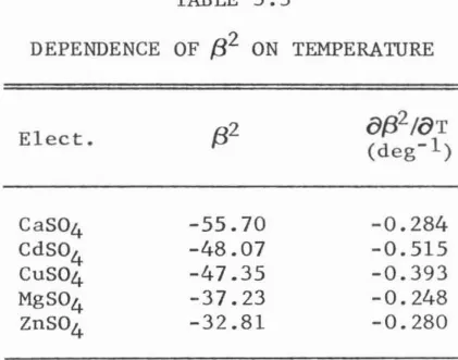
Dependence of

p

2

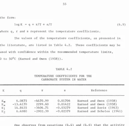
on Temperature

Chemical Reactions and Equilibrium Equations for the Carbonate System in Water

Temperature Coefficients for the Carbonate System in Water

Equipment and Instruments Used in the Experimental Procedure

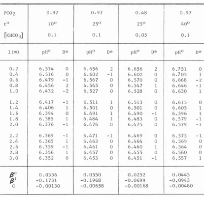
pRo Values in KHC03-KCl Solutions pRo Values in NaRC03-NaCl Solutions

pR0 Values in KCl-R2C03 and NaCl-R2C03 Solutions at 25°C

~pRo Values for MCl-R2C03 Solutions at 25°C pRo Me_{asurements in NR4Cl-R2co 3 Solutions} pR0 Values in CaCl2-R2C03 Solutions at 25oc pR0 Values in MgCl2-R2C03 Solutions at 250C Summary of the MHC03 Virial Coefficients Average ~{J/~T of MHC03 Electrolytes

Measured pR0 Values in the System~' Na+-RC03-, Cl-Comparison of Experimental pR0 Values

Thermodynamic Solubility Product of Gypsum at 25°C

Table 5.2

5.3

5.4

5.5 A.la A.lb A. 2 A.3a A.3b A.3c A.3d

A.4

A.5

Title

Thermodynamic Solubility Product of Gypsum from

0.5 to 6ooc

The Thermodynamic Solubility Product of Calcite at 25°C

Solubility Properties of Calcite and Gypsum in a Lake Water

Osmotic Properties of Seawater and Product Water Y Values of Some 1:1 Electrolyte Solutions

Y Values of Some 1:1 Electrolyte Solutions

Y Values of Some 1:1 and 1:2 Electrolyte Solutions Y Values of Some 1:2 Electrolyte Solutions

Y Values of Some 1:2 Electrolyte Solutions

Y Values of Some 1:2 Electrolyte Solutions

Y Values of Some 1:2 Electrolyte Solutions Y/X1 Values of Some 2:2 Electrolyte Solutions Y Values of Some 2:2 Electrolyte Solutions

Page

94

96

98 100 102 103 104 105

106

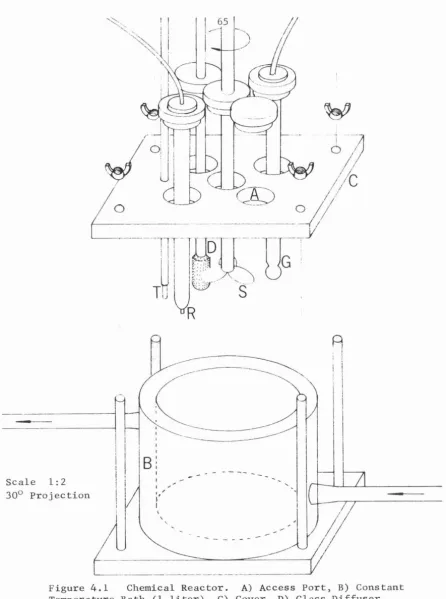
[image:8.584.93.493.87.481.2]

Figure

3.1

3.2 3.3

3.4

3.5

3.6

3.7

4.1

4.2

LIST OF FIGURES

Title

Y vs.

x

_{1 Values for 1:1 Electrolytes} Y vs. X1 Values for 1:2 Electrolytes

Temperature Variation of the First and Second Virial Coefficients of 1:1 Electrolytes

Temperature Variation of the First and Second Virial Coefficients of 1:2 Electrolytes

Y/X1 vs. X2/X1 for 2:2 Electrolytes Y vs. X1 Values for MgS04

Temperature Variation of the Second Virial Coefficient of 2:2 Electrolytes

Chemical Reactor

Temperature Variation of the First and Second MHC03 Virial Coefficients

Page 36 37

39

40

46

48

50

65

Roman Capital Letters

A Debye-Huckel coefficient B Interaction function C Third virial coefficient D Finite pH difference E pH calibration error

Gex Excess Gibbs energy of mixing I Ionic strength

I* Pseudo-ionic strength

J Apparent molal heat capacity

K Thermodynamic dissociation constant Kip Thermodynamic ion product

Ksp Thermodynamic solubility product L Relative partial molal enthalpy M Specific cation

M1 Molecular weight of solvent P Pressure

R Gas constant S Solubility ratio T Absolute temperature

W Power consumption/flow rate X Specific anion

Roman Lower-Case Letters

a, a'

c, c'

d

e f

g

m

Any anion in solution

Activity of water

Coefficient

Any cation in solution

Coefficient

Coefficient

Debye-Hlickel function

Ionic strength function

Molal concentration

q, r, s Coefficients

t Temperature in °C

v 1 Partial molal volume of water

Greek Letters

a Coefficient

P

Virial coefficient

Y

Activity coefficient

6

Incomplete dissociation factor

E Dielectric constant of water

8

Like-charge virial coefficient

V Number of moles

17

Osmotic pressure

a

Standard deviation

¢

Osmotic coefficient

¢

J

Molal heat capacity ¢L Apparent molal enthalpy

~ Triplets interaction coefficient

n

Osmotic membrane constant

Operators

[

J

Molal concentration

( ) Molal activity

E

Summation

~ Difference

Chapter 1

INTRODUCTION

1.1 The Bicarbonate Ion as a Main Component of Natural Waters

The bicarbonate ion is commonly found in natural waters, and its

intrinsic properties are of importance in the study of water chemistry

equilibrium. Some of the basic chemical and physical properties of

this anion are reviewed below.

In nature the bicarbonate ion leaves or enters a solution via

one or more of many mechanisms. Among these are the processes of

photosynthesis-respiration, contact with the atmosphere and

precipitation-dissolution of carbonate and bicarbonate minerals. Due

to the common occurrence of these processes the bicarbonate ion is a

ubiquitous component of natural waters.

The bicarbonate ion exhibits amphoteric properties in aqueous

solutions, being the intermediate state of protonation of the carbonate

system. These important properties are directly related to the acid

and base neutralizing capacities of aqueous solutions. Often in nature

the bicarbonate ion is the main acid-neutralizing agent of the water

(i.e., alkalinity). The pH of a water solution is therefore dependent

on the concentration of bicarbonate ion.

Several thermodynamic models have been proposed to evaluate the

intrinsic characteristics of mixed electrolyte solutions. The general

following section. Natural waters may be considered as aqueous multi-component electrolyte solutions and therefore may be studied as such. Quantitatively, the concentration of the individual ions in natural waters varies widely from place to place, but their main components are usually the same. In natural waters the most commonly found cations are H+, Na+, K+, ca2+ and Mg2+, and in polluted waters NH4+. The anions usually present in natural water are oH-, cl-, HCOJ-, No₃-, H2P04-, F-, S04 2-, C03 2 -, HP04 2- and P043 -. Therefore, the equilibrium properties of bicarbonate in natural waters may be studied by consider-ing HC0 3 as an individual component in a mixed electrolyte solution. A method is proposed in this work to evaluate accurately some important equilibrium characteristics of the bicarbonate ion in natural waters.

1.2 Thermodynamic Models

Several thermodynamic models have been proposed to predict the activity coefficients of mixed electrolyte solutions. These models give reasonable results for relatively simple multicomponent systems; however, few of them may be utilized in the calculation of the activity coefficients of electrolytes having more than four different ions in solution. The two most common methods of evaluating activity coeffi-cients of such complex electrolytes are the Ion Association Model and the Ion Interaction Model. The general characteristics and basic assumptions of these equilibrium models are presented below.

Association Model, which assumes the formation of ion pairs by

oppo-sitely charged ions (i.e., counter-ions). The Br~nsted-Guggenheim Ion Interaction Model is the alternate procedure employed in the evaluation

of several thermodynamic properties of aqueous solutions, including the activity coefficients of the individual ions in solution. The latter

method approaches this problem by assuming interactions among the ions

in solution.

The activity coefficient of any solute is defined as the

dimen-sionless ratio between its activity and concentration in solution.

Under very dilute conditions this ratio approaches unity. Stumm and

Morgan (1970) report that the Debye-Huckel theory, which considers only long-range electrostatic interactions between the ions, is accurate in

most cases for ionic strengths below 0.01 M. Deviations from the ideal

Debye-Huckel theory at higher ionic strengths are attributed to short

-range interionic forces. Different assumptions are used by the two basic models to account for deviations from ideality in concentrated

solutions.

The Ion Association Model assumes that deviations from the

Debye-Huckel theory are caused by differences in the ion sizes and/or

by the relatively strong binding of counter-ions to form ion pairs.

According to this model, the concentration of a specific type of ion

pair is directly proportional to the activity of its free counter-ion

components. The ion association criterion implies, then, a distinction

between the thermodynamic properties of both free ions and ion pairs.

con-sideration the presence of ion pairs, complicates considerably the

equilibrium calculations of mixed electrolyte solutions. Furthermore, tedious approximations have to be executed in order to satisfy the electroneutrality and mass balance conditions.

Several al ternate methods are used in the Ion Association Model to compute the activity coefficients of free ions in solution. The following methods are widely used in the computation of these

param-eters:

i) The extended Debye-Huckel equation, and ii) The Mean Salt method (Macinnes convention) .

The first method, which utilizes an adjustable parameter (ion size param-eter), permits one to evaluate analytically the activities of the in-dividual free ions. The accuracy of this method is dubious at ionic strengths above O.OSm, and should be used cautiously in concentrated solutions.

The Mean Salt method for obtaining the individual free ion

activity coefficients has lately come under strong criticism. By con-vention, this method assumes that the activity coefficient of the potassium ion is equal to that of the chloride ion at a given ionic strength, regardless of the nature of the other ions in solution. Whitfield (1974a),mentions,among others, the following disadvantage of

of this method:

"The widely employed Macinnes convention is ambiguous at ionic strengths greater than 0.1 M and contradicts anum-ber of conventional definitions of single ion properties in implying that the activity coefficient of the chloride ion is the same in all solutions of alkali and alkaline

A thermodynamic property of aqueous solutions, which is not well

understood, is the ion-pair activity coefficient. A great number of

techniques have been proposed to evaluate this parameter. The lack of

common grounds for the computation of the activity coefficients of ion

pairs is directly reflected on many other thermodynamic properties of

the solution as a whole.

Finally, in order to compute accurately the free ion activity

coefficients, i t becomes necessary to know precisely the value of the

ionic strength of the solution. Some researchers who utilize the Ion

Association Model evaluate the ionic strength of a solution by adding

the individual contribution of free ions to the contribution of ion

pairs. Other investigators claim that this is incorrect and evaluate

this parameter from the contribution of the individual ions' total

con-centrations. This discrepancy may lead to wide differences in the

pre-dicted value of the activity coefficients of both free ions and ion.

pairs.

The osmotic and activity coefficients of single electrolyte

solutions may be accurately predicted by the use of the Ion Interaction

Model. These parameters are evaluated by the addition of an

inter-action term to the Debye-Huckel function. (This theory is studied in

more detail in the next chapters.) The interaction term is a

semi-linear relationship of the molality of the solution, which

rapidly tends to linearity as the concentration of the electrolyte

increases. At a fixed temperature and pressure the slope of the

absolute value (i.e., deviation from ideality) is usually higher for multivalent electrolytes. Both the osmotic and activity coefficients

of mixed electrolytes may be accurately predicted by assuming that the

multiple interactions upon a specific ion are additive (Lewis and

Randall (1961)).

The simplest method to predict short-range interactions among

the ions is to assume linear i ty in the ion interaction term. This approach has yielded reasonable results for the activity coefficients

of systems as complex and concentrated as sea water (Whitfield (1973)). Recently Pitzer (1973) has proposed a more detai led, but at the same

time more complex, approach for the description of the osmotic and

activity coefficients of single electrolytes from infinite dilution to

6.0 m. The value of the interaction term in Pitzer's method is de-scribed by three virial coefficients which multiply an equal number of functions of the ionic strength of the solution. Pitzer and Mayorga (1973) have evaluated and published the values of the virial coeffi-cients of over 200 1:1, 1:2 and 1:3 electrolytes. The evaluation of

these coefficients was performed from measurements of the activity and

osmotic coefficients of single electrolyte solutions. In another

pub-lication Pitzer and Mayorga (1974) propose a mathematical approach to

the evaluation of these two thermodynamic properties in solutions con-taining 2:2 electrolytes.

between like-charged ions as well as triple-ion interaction. Higher order electrostatic terms for multivalent electrolytes may be described by the technique proposed by Pitzer (1975). Many ambiguities existing in the theory of strong acids may be resolved by using Pitzer's method in the analytical studies of these electrolytes (Pitzer and Silvester (1976)).

1.3 Evaluation of the Thermodynamic Models

The main objection to the use of the Ion Interaction Model in aquatic chemistry is the execution of lengthy mathematical manipula-tions, but the accuracy of the model more than compensates this objec-tion. In single electrolyte solutions the calculations involved in the Ion Interaction Model are probably more complex than those required by the Ion Association Model. However, for mixed electrolyte solutions, the opposite condition is often observed. This condition is due to the cumbersome approximations necessary to satisfy both the mass balance and electroneutrality constraints in the Ion Association Model.

1.4 Thermodynamic Properties of M-HCOJ Salts

In view of the chemical importance of the bicarbonate ion in natural waters i t becomes necessary to describe its thermodynamic be-havior by means of a sound equilibrium model. The model chosen in this work was the Ion Interaction Model utilizing the latest modifications by Pitzer and co-workers.

Many investigations have dealt with the problem of predicting the activity coefficient of the bicarbonate ion in the presence of various cations. Nonetheless, most of these investigations have dealt with the problem according to the Ion Association Model. The validity of this approach is directly related to the prediction accuracy of the free bicarbonate ion activity coefficient. This parameter is usually evaluated by means of either one of two techniques: by the extended Debye-Huckel equation or by interpolation of tabulated values. A pre-vious discussion of the effectiveness of the first technique to describe activity coefficients reveals that its validity is limited to very

dilute solutions. The tabular values of the free bicarbonate ion

In lieu of the Ion Association Model, Butler and Huston (1970)

have studied the activity of HC03- in NaCl solutions according to

Harned's Rule. Harned's Rule reduces to the simplified Interaction

Model at high ionic strengths. Other than this study little is known

about the interaction properties of the bicarbonate ion in natural

waters.

This dissertation presents a theoretical approach to the

deter-mination of the virial coefficients of HC03- in natural waters at

various temperatures. Based on this approach the virial coefficients

of various bicarbonate salts are evaluated from experimental results.

These salts included the following bicarbonate compounds: NaHC03,

KHC03, NH4HC03, Ca(HC03)2, and Mg(HC03)2. The cations of these salts

are the most important positively charged ions in natural and polluted

waters. Thus, the knowledge of their respective interaction

character-istics permits a more precise understanding of the equilibrium

condi-tions of most water bodies.

1.5 Effects of Temperature on Aqueous Solutions' Equilibria

Local, seasonal and diurnal temperature variations are often

observed in most natural phenomena. Temperature changes are of special

interest in natural waters because, in general, their thermodynamic

properties are temperature dependent. An example of these properties is the ion activity coefficient, which has a strong temperature

-trostatic function and the short-range interaction term are temperature functions.

Chapter 2

THE ION INTERACTION MODEL

2.1 Literature Review

The Ion Interaction Model was originally developed by Br¢nsted

(1927) who proposed that the thermodynamic properties of aqueous solu-tions could be evaluated from the interactive forces between the ions in solution. He assumed that interactions between oppositely charged ions would be dominant, thus neglecting like-charge ion interaction. Guggenheim (1936) made a distinction between the two terms in the acti-vity coefficient equation: the electrostatic interaction function and the short-range interaction term. He described the first function by

the Debye-HUckel equation, which he assumed depended only on the ionic strength and the temperature of the solution. He also assumed that the second term might be described by a polynomial function in concentra-tion with a linear leading term.

The emphasis of more recent publications has been the study of the short-range interaction term. Many researchers, including

Guggen-heim and Turgeon (1955), and Lewis and Randall (1961), have used a sim-ple approach to this problem. They have assumed that the interaction term may be described by a linear function in concentration. Whitfield

may be observed at low ionic strengths.

Pitzer (1973) has developed a mathematical model which takes

into consideration deviations from linearity. By considering like -charge interactions Pitzer and Kim (1974) have obtained excellent agreement between calculated and experimental measurements of the acti-vity and osmotic coefficients of mixed electrolytes. The theory deve l-oped by Pitzer (1973) for the Ion Association Model appears to be the most accurate technique for predicting the equilibrium conditions of mixed electrolytes. The basic principles of Pitzer's theory, along with some temperature considerations, are presented in this disse

rta-tion. For more detailed information the reader is referred to the

original publications.

2.2 General Equations

By convention, the ionic strength of a mixed electrolyte

solu-tion, I, is defined as follows:

where mi represents the molal concentration of any ion i in solution, and

Zi represents the valence of any ion i in solution.

(2.1)

The osmotic coefficient of a solution is intimately related to various thermodynamic properties of its component solvent and solutes. The activity coefficients of the solvent and the ions in solution are,

to the importance and interdependence of these thermodynamic proper-ties, a detailed study of the osmotic coefficient of mixed electrolyte solutions is presented in this dissertation.

Based on the Ion Interaction Theory, Pitzer and Kim (1974)

pro-pose the following equation for the osmotic coefficient,

¢,

of a mixed

electrolyte solution:

where

¢-

1

£~

=

1

LID·

_{• l.}

J..

+

{"'a

f.

m ••

[e ••.

+

16~.·

+

f"'c

lfrcaa'

J

l

1

+

L2jf

(Debye-Hlickel function)

(2.2)

(2.3)

A represents the Debye-HUckel coefficient. This coefficient

is a function of the temperature of the solution, T, and

is equal to 0.392 at 25°C, ~ o

+

{Jl

-a11f

B111:x

=

/J

111:x MX e

(2.4)

c, c' and M represent the names of the cations in solution, a, a' and X represent the names of the anions in solution.

represents the total molal charge of the solution,

C represents the third virial coefficient,

0

represents the interaction coefficient between like-charge ions.

8'

""

88/f)

I

(2.5)

~ represents the interaction coefficient for triplets.

a l equals 2.0 for 1:1, 1:2 and 1:3 electrolytes, or

0I

equals 1.4 for 2:2 electrolytes.

The virial coefficients of 227 pure aqueous 1:1, 1:2 and 1:3 electrolytes at 25°C are evaluated and presented by Pitzer and Mayorga

(1973) . Numerical values for some like-charge and triplets inter-action coefficients are listed by Pitzer and Kim (1974).

The long-range interaction effects on the osmotic coefficient

of a solution are mathematically simulated by the Debye-Huckel function, which is represented by the first term in equation (2.2). The remaining

terms in this equation simulate the short-range interaction effects on the osmotic properties of a solution.

Two important thermodynamic properties of aqueous mixed elec -trolytes, the osmotic pressure of a solution and the activity coeffi-cient of the solvent, may be computed from the osmotic coefficient of

the solution. Lewis and Randall (1961) propose the following two equations for the osmotic pressure of mixed electrolytes,

11

,

and the

activity of water, a 1:

ll

=

=

-M1

1000

Ml

1000

(2.6)

where R represents the gas constant and equals 1. 98726 cal/°K - mole, T represents the absolute temperature in Kelvin degrees, v

1 represents the partial volume of water. (v 1

=

18.0 cc/mol for an infinite dilution at standard temperature and pressure.) M

1 represents the molecular weight of the solvent (18.0g/mol for water).

An electrolyte composed of a cation M with valence ZM and an anion X with valence Zx dissociates in water according to the reaction

(2.8)

where VM represents the number of cations of M per molecule of MX, and

Vx represents the number of anions of X per molecule of MX.

To satisfy the electroneutrality condition of the electrolyte MX i t is necessary that

(2.9)

The activity coefficient of the electrolyte MX in solution,

YMX>

is computed from the geometric mean of the activity coefficient

of the cation

YM

and the activity coefficient of the anion

Yx :

(2.10)

where (2 .11)

Based on the Ion Interaction Theory, Pitzer and Kim (1974)

electrolyte MX in a multicomponent solution. This equation may be

easily resolved by symmetry into its two individual components, the

activity coefficients of the cation and the anion. The two equations

obtained by this procedure are presented below:

+

and

ln

Yx

+

\~me~ me' ( 1,/tee 'x e e'

z2

~·

ma'

()~a'

+

X

l:ma 2 a

where f

B I pl '

MX "" 81 {1)

+

z

2 ()'

x ee'

)

2

1.2 ln (1

+

1.2

,fl>]

(2.12)

(2.13)

(2.14)

(2.15)

2

(2.17)

=

Seemingly, the equations to calculate the osmotic and

acti-vity coefficients of a solution are very lengthy. Nevertheless, i t

must be remembered that at the given ionic strength of the electrolyte

solution,

f~,

f, g₁ and

g~

are constant. Therefore, the Ion

Interaction Model is a simple and accurate technique to calculate the

equilibrium properties of mixed electrolyte solutions.

The above equations are somewhat simplified in the case of the

dissolution of a single electrolyte. Since only one anion and one

cation are present in this type of solution, the contributions of

0,

0'

and ~ are non-existent. The equations which describe the

thermo-dynamic properties of pure salt solutions are given by Pitzer and

Mayorga (1973). It was previously mentioned that these authors re

-port the values of the first, second and third virial coefficients of

227 1:1, 1:2 and 1:3 electrolytes. These parameters were obtained by least square analyses of various thermodynamic proper t ies of single

electrolyte solutions.

Pitzer and Kim (1974) suggest that in most practical cases

8

may be assumed to be constant over the ionic strength. In other words,

they assume

0'

to be equal to 0. Based on the above assumption they

are able to predict accurately the activity and osmotic coefficients

~utilized in such predictions.

The effect of

8'

on the thermodynamic properties of most mixed electrolytes is minor. However, if maximum accuracy is desired in the prediction of these properties i t becomes necessary to consider the variation of

8

with the ionic strength. For complete information on

the dependence of the like-charge interaction coefficient with ionic strength, the reader is referred to work of Pitzer (1975).

2.3 The Ion Interaction Theory for 2:2 Electrolyte Solutions

The capability of an electrolyte to completely dissociate in a solvent is directly related to the electrostatic attraction between the counterions in solution. Obviously, this electrostatic attraction in-creases as the absolute value of the counterions' charges increase. The model presented thus far may be used to describe the thermodynamic properties of electrolyte solutions only in the case where the absolute values of the valences of one or both counterions are equal to one. The particular case of 2:2 electrolytes (which do not completely dis-sociate in aqueous solutions) is considered in this section.

The osmotic coefficients of various single divalent cation sulfates at 25°C, as experimentally determined by various researchers, were summarized by Pitzer (1972). These coefficients were successfully predicted by Pitzer and Mayorga (1974) by means of an interaction model, which takes into consideration incomplete electrolyte

the B¢, B and B' equations. Even though this approach gave excellent

results for single divalent cation sulfates i t failed to predict their

solubility product in seawater (Whitfield (1975a,b)). In these

publi-cations Whitfield utilizes a hybrid model (a combination between the

Ion Association Model and the Ion Interaction Model) which permits a

reasonable explanation of the difference between measured and

calcu-lated solubility products of sulfate salts in seawater. The hybrid

model proposed by Whitfield assumes simultaneously Pitzer and Mayorga's

compensation for ion association, as well as the existence of ion pairs

as individual entities.

Three conclusions may be drawn from the above works:

a) Pitzer and Mayorga's interaction model for incomplete

dis-sociation of divalent cation sulfates in aqueous solutions

works satisfactorily in the case of single salt solutions,

but fails to predict the thermodynamic properties of such

sulfate salts in mixed electrolyte solutions.

b) The inclusion of the extra interaction term in Whitfield's

hybrid model is redundant, for the purpose of this term is

to compensate for ion association.

c) The simplicity of the Ion Interaction Model is destroyed

when the particular problem of incomplete dissociation is

approached from the point of view of ion association. In

other words, if a hybrid model is utilized (by considering

ion pairs as individual components of the solution) tedious

balance and electroneutrality conditions of the solution.

A modification to Pitzer and Mayorga's work is proposed in

this dissertation. This modification permits one to compensate for

incomplete dissociation without implicitly considering ion pairing.

The thermodynamic solubility product of gypsum (i.e., CaS04 · 2H

20) in

a variety of mixed electrolyte solutions is studied in Chapter 5. The

prediction accuracy of this thermodynamic constant confirms the

vali-dity of the proposed modification. Following is presented the

pro-posed Ion Interaction Model for 2:2 electrolyte solutions.

The activity of an individual ion is reduced by a factor

6

if

incomplete dissociation occurs. The value of this factor varies from

unity for complete dissociation, to zero for nil dissociation. It is

assumed in this dissertation that 2:2 electrolytes in solution

asso-ciate to some extent, while 1:1, 1:2 and 1:3 electrolytes do not ex

-perience this phenomenon. The following empirical equation is p

ro-posed for

6

:

where

(2.19)

i represents the divalent cation M or the divalent anion X,

j represents the divalent anion X or the divalent cation M,

p

2 _{represents the association virial coefficient, which must}

be determined experimentally,

I* represents the pseudo-ionic strength of M and X. I .e.,

and _[ 1 - ₍ 1

+

a

₂

vi

r;;:

*

-

«

z

₂

~I*

)

e

-

o2«

]

(2.21)

Thus, the individual ion activity coefficient, compensated for incomplete electrolyte dissociation,

Y

!,

may be computed as follows:

(2.22)

An extra term must be added to the B~ equation to compensate the osmotic coefficient for incomplete electrolyte dissociation. The proposed equation is as follows:

(2.23)

Values of

p

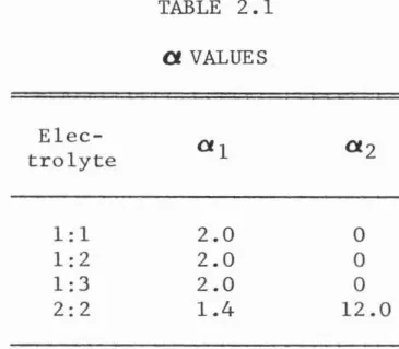
2 for various divalent cation sulfates are presented in Pitzer and Mayorga's work. The values of a, which are also those recommended in the aforementioned work are listed in Table 2.1.

Elec

-trolyte

1:1 1:2 1:3

2:2

TABLE 2.1

a

VALUES

2.0 2.0 2.0

1.4

0 0 0 12.0

[image:33.584.202.385.411.571.2]

that due to the large value of a2, the exponential terms in both

equa-tions (2.21) and (2.23) rapidly tend to zero as the ionic strength

in-creases. In relatively concentrated single electrolyte solutions

(I> O.lm) the equations proposed in this dissertation predict that the effect of

P

2 on the solution osmotic coefficient is nil, while this effect reduces the ln

Yi

by a constant equal to 2

P~j

mj/Ct~

I*

Experi-mental measurements of the osmotic and activity coefficient of divalent

cation sulfate solutions confirm these trends (Pitzer (1972)).

2.4 Example

The purpose of the numerical example in this section is to

apply the Ion Interaction Model in order to calculate the thermodynamic

properties of a mixed electrolyte solution.

Statement: Marshall and Slusher (1966) report that the

solu-bility of gypsum (Caso₄ • _2H2o) in a 0. 548 m NaCl solution at 25°C is 0.0372m/l. Calculate the thermodynamic solubility product of gypsum.

Solution: The molal concentrations of the ions in solution

are: 0.548

and _mea

=

_mS04 0.0372.

The ionic and pseudo-ionic strengths of this solution are, according to equations (2.1) and (2.20), respectively:

I

=

~Xm..z? _{1.-A.. l.} = 0.6968m

I*-~

(

mMzM

2

+

mxz/)

= 0.1488m

(i.e., Na, Ca, Cl,

so

_{4 ),} M represents Ca and X represents S04.

The functions f(I), and

f~

may be computed from equations (2.14) and (2.3) respectively (at 25°C A 0.392):

f - A

[

Ji

+

2 ln (1

+

1.2 ..jf)

J

1 + "1.2Jf 1.2 -0.6169

f~ ... - AJr

1

+

L2Ji

-0.1635

The functions _{g 1 (I),} g₁' _{(I), and g 2} (I>'<) are then computed from equations (2.17), (2.18) and (2.21) respectively. The values of ~ and

a

₂ (which are presented in Table 2.1) and the previously

calcu-lated magnitudes of I and I* are the input parameters for these equations.

gl (I)

0.3568 for a₁ 2.0 0.4774 for

a

₁ 1.4

a

1

~I

2

[-

1

+ (

1

+

a

1

.[I

+

~

eel

2 I ) e-a,.ff

J

-0.2417 for

a

₁ 2.0 - 0. 2391 for

a

₁ 1.4

2

0.0980 for

a

₂ = 12.0

M X

p

o

pl

p

2

c

Na Cl 0.0765 0.266 6.4 X lQ-4

Na

so

₄ 0.0196 1.113 2.0 x lo-3>'<

Ca Cl 0.3159 1.614 -1.2xlo-4

Ca

so

₄ 0.2000 2.650 -55.7 0.0

>'<Improved value by Pitzer and Kim (1974)

The values of most like-charge and triplet interaction

coeffi-cients, which are required in this example, are given by Pitzer and

Kim (1974) and Downes and Pitzer (1976). These values are as follows:

8Na,Ca 0.000

8_c1,

so

4 -0.020

1/f,

Na,Cl,S04 0.004

1Jf,

Na,Ca,Cl 0.000

The B ~~>, B, B' and

6

parameters are described by the next four

equations (equations (2.23), (2.15), (2.16) and (2.19) respectively):

1/>

BMX P~.

+

pl

MXe -a1

fX

+

p2

Mxe -a2.{F

BMx

P~x

+

P~.

gl (I)

B:.x

pl

gi

(I)

lnc5i

=

/J~jm

.

g

(I*)

l. J 2

The results obtained by applying these equations to the mixed

M X BcP B B'

Na Cl 0.127 0.172 -0.045

Na

so

₄ 1.878 0.417 -0.187

Ca Cl 3.010 0.892 -0.272

Ca

so

₄ 1.021 1.465 -0.441

ln6ca

=

ln6₈₀ -0.2031 4

In order to solve the stated problem i t is not necessary to com-pute the activities of the sodium and chloride ions. Therefore, only

the activities of the calcium and sulfate ions are calculated in this

exercise. The osmotic coefficient of the solution and the activity of calcium and sulfate may be computed from equations (2.2), (2.12) and (2.13) respectively. The net effect of 8' on the calculated osmotic and activity coefficients is usually minor, and for most practical ap-plications may be ignored. Without much loss of accuracy one may assume that

8'

and the unavailable ~values are equal to zero. There-fore, the osmotic coefficient of the solution, and the uncompensated activity coefficients of the calcium and sulfate ions are computed as

¢-

1

Therefore,

¢

+

+

1

Em-

.

~

~

EmcE,

me'

c c

..Ema

E

ma' a a' -0.09961

0.90039

[Bee'

+~,+

0

~rna

Wee' a ]

[e ••.

+y(:·

0

+

fmc 11tcaa' ] )

zM2 f

+

2~ma

_{[ BMa}

+

(

_{fmcZc ) CMa}

J

+

2.,EmC6MC

+

.Erne ..Ema ( ZM2

B~a

+

ZMCc

+

1/JMca

c c a a .

l:i

..Ema ..Ema' (

~0

+

1/JMaa'

+

Z a a'

a a'

1.5063

= - 2.0638

)

M Ca

X so

4 c Na, Ca c' Ca, Na a

=

Cl, so₄ a' so

4, Cl

i Na, Ca, Cl, so₄

The compensated activity coefficients of the calcium and sul-fate ions are computed by inserting the appropriate values into equation (2.21):

ln~

ln

Y.

+

ln6.

I

1.7094 for i Ca

=

]. l.

2.2669 for i so₄ Therefore, y c

Ca 0.1810 "so4 0.1036

The activity of the solvent, water, may be evaluated from the

knowledge of the solution osmotic coefficient and the molality of the species in solution. From equation (2.7) one obtains:

Therefore,

Ml

¢J;'!llj_

1000 ].

- 0.0190 0.9812

(where M₁ 18.0)

Ksp m

ca

m

so4

y

ca

c

Y.

sco4

a2l (2.24)

Chapter 3

TEMPERATURE EFFECTS ON THE THERMODYNAMIC PROPERTIES OF ELECTROLYTE SOLUTIONS

3.1 Thermal Effects on Electrostatic Interactions

The thermodynamic properties of aqueous solutions are usually strongly dependent on temperature. The assumption that natural waters may be treated as mixed electrolytes under ideal conditions of

stand-ard temperature and pressure is often incorrect. Although pressure variations are of importance in chemical equilibrium, such variations

are of little importance in the study of surface waters, which are the

main concern of Environmental Engineering. The scope of this chapter is the study of the temperature effects on the thermodynamic

equili-brium properties of aqueous solutions at one atmosphere total pressure. Literature information on the temperature effects on

electro-lyte solutions equilibria is abundant. This information is usually

analyzed from the Ion Association Model point of view. Perhaps one of

the most complete works in this area is that of Helgeson (1967), who

calculates several thermodynamic properties of various electrolyte

Interaction Model is utilized to estimate thermal effects on Br~nsted acids' equilibria.

The Ion Interaction Model may be used to describe the thermo-dynamic proper t ies of aqueous solutions at variable temperatures. Lewis and Randall (1961) conclude that both the long-range

electrosta-tic attraction and the short-range interaction between ions in solution are temperature dependent. The electrostatic attraction terms for the osmotic and activity coefficients may be computed from equations (2.3)

and (2.14) respectively. The only temperature dependent parameter in these equations is the parameter A, which has a triple dependence on temperature. This parameter is a direct function of temperature, the

solvent dielectric constant and the coefficient of thermal expansion of the solvent (Lewis and Randall (1961)). The effect of temperature on

the volumetric expansion for water is unimportant when compared with the two other dependences, and i t is ignored in this disser tat ion.

The dielectric constant of water may be expressed as a poly-nomial function of temperature. A least-square criterion for curvi -linear regression may be utilized to evaluate the coefficients of this

polynomial. Utilizing the above criterion to fit a third-degree poly-nomial to the tabulated values of the dielectric constant of water

(Weast (1975)), the following equation is obtained:

where

E = 87.924- 0.40873t

+

1.01465 X l0-3 t 2 - 1.9365 X l0-6 t 3 (3.1)

E represents the dielectric constant of water, and

t

=

T - 273.16 (3. 2)

The coefficients in equation (3.1) are in close agreement with the values reported ear l ier by Harned and Owen (1958). The equation which describes the dependence of A with respect to temperature is given below (Robinson and Stokes (1959)):

A 1.400 X 106

(ET)3/2 (3.3)

The temperature effects on the long-range electrostatic inte r-action terms (in the osmotic and activity coefficients equations) may be calculated by means of the three above relationships and equations (2.3) and (2.14). These thermal effects are often of higher magnitude than the ones observed for the short-range interaction terms. Follow-ing is presented a thermodynamic analysis of these secondary tempera -ture effects on the activi ty and osmotic coefficients of electrolyte solutions.

3.2 Thermal Effects on Short-Range Interactions

Several thermodynamic parameters are intimately related to the temperature effects on the interactive properties of ions in solution. Direct or indirect measurements of these properties may be utilized to compute the dependence of short-range interactions with respect to

Pitzer and Mayorga (1973) propose the following relationship for the excess Gibbs energy of mixing of single electrolyte solutions:

where

4AI

1.2 1n (1

+

1.2

/i)

+

2m2 V.,.llx [

P~x

+

P~x

g1 (I)

+

P~x

(

&2 (I*)

3

+

2m Z11 1111 C11x

Gex represents the excess Gibbs energy of mixing, m represents the molality of the solution, and

I* equals I for single electrolyte solutions.

(3.4)

The excess Gibbs energy of mixing is related to the relative apparent molal enthalpy of an electrolyte in solution by the fol lowing partial differential equation:

1 8(Gex/T)

m 8(1/T)

T,m

(3. 5)

where ¢L represents the apparent molal enthalpy of an electrolyte in solution relative to infinite dilution.

Combining equations (3.4) and (3.5) one may express the tern-perature variation of the virial coefficients as a function of ¢L:

1

2

2m

v.,.vx

T

=

{

aP?.x

+

{)T

{

~

+

3.333....!.. ln(l

+

1.2

../i)

m

8/J~x

g(I)

+

O~x

(

g2 (I*)

8T

OT

8A

8(1/T)

acMx

l

8T

IT

(3. ~)

ob-ably even of less importance . I t is therefore assumed in this work that

8

C/

8T

=89/8T =81/f/()T

=

0. Assuming no variation of the C

virial coefficient with temperature, equation (3.6) may be represented by a linear polynomial of the form:

where

y

y

bo

+

bl xl

+

b2 x2

represents the left side terms of equation (3.6),

(3. 7)

x₁ and x₂ represent the respective functions of I and I* in equation (3.6), and

b₀ , b1 and b2 representi:}(3°/CJT,

8f3

1/()T and

8{3

2

/i}

T

respectively.

It is important to remember that

{3

2 represents the ion pairing virial coefficient. In this study this coefficient differs from zero

only in the case of 2:2 interaction. Thus,

of3

2

/8T

is equal to zero

for 1:1, 1:2 and 1:3 electrolyte solutions. For such solutions, graphs of Y with respect to _{x 1 should yield} points lying on straight lines in which the intercept, b₀ , represents

8{3

°

/8T

and the slope of the line,

b 1 , represents

8{3

1

/i}T.

This graphical technique permits one to evaluate

r eadily the variation of the first two virial coefficients with re -spect to temperature. A more complete graphical method, which permits the simultaneous evaluation of b_{0 ,} b₁ and b

2 for 2:2 electrolyte sol u-tions, is discussed later in this section.

Another important thermodynamic property, the relative partial molal enthalpy of an electrolyte in solution, is related to the

activ-ity coefficient of the electrolyte as follows:

where represents the partial molal enthalpy of an electrolyte

in solution relative to infinite dilution.

In single electrolyte solutions, the rate of variation of the

virial coefficients with respect to temperature may be also computed

from experimental measurements of L. This is obtained by

differen-tiating the individual components of equation (2.10) with respect to

temperature. Then by rearranging the terms in equation (3.8), the

following expression is obtained:

"

l

L

z,.zxl

[

Vf

2 ln ( 1

+

1. 2

,{f)

J

l

T

4mV,.Vx VRT

+

1+1.2Vf

+

1.2

= a8~1

+

a~~!

( g, (I)

+

e-a,.rr

)

aT

8T

2

(3.9)

If the last term in the previous expression is ignored, this

expression may be represented by a linear polynomial of the form of

equation (3.7). Obviously, the values of Y,

x

₁ and

x

2 are those

of their corresponding functions in equation (3.9). As in the

pre-vious case, plots of Y against

x

₁ values (for 1:1, 1:2 and 1:3 elec-trolyte solutions) should yield points on straight lines. The

signi-ficance of the slope and intercept of the lines is the same as before.

Theoretically, the second derivative of the virial coefficients

with respect to temperature may be evaluated if either the relative

partial molal heat capacity or the relative apparent molal heat

capa-city are known. The respective equations for these two thermodynamic

(3.10) J

and (3.11)

where represents the molal heat capacity relative to infinite dilution, and

J represents the apparent molal heat capacity relative to infinite dilution.

Literature information on the numerical values of the heat capacity functions is rather limited. This information suggests that the variations of

¢L

and

L

with respect to temperature are small in com-parison with their respective values, and for most electrolyte~ they

may be ignored. I t is assumed throughout this dissertation that both

¢L

and

L

do not vary with temperature. In other words, i t is assumed that the second partial derivatives of the virial coefficients with respect to temperature are equal to zero.

The functions Y,

x

1 and

x

2 in equation (3.7) may be evaluated from their respective terms in equations (3.6) and (3.9). The nume ri-cal values of Y,

x

_{1 and}

x

_{2 for some important} electrolytes are prese n-ted in tabular forms in the Appendix. Experimental results of

¢

L

and

L

at various ionic strengths are repor ted in several literature sources. Y values (computed from the experimental results of the 1:1 and 1:2

electrolytes listed in the Appendix) are plotted in Figures 3.1 and 3.2 respectively. As expected, the data points follow a linear correlation,

150 100 50

0

-50

(oK-1)

I

iO

I

I

l

6 6. 6. 6,. 6.

~.a•.

.

.

...

.

'T!1>

I>

I>

l>ot o

~

.2.

~

f

t

~

$

o~

~

~o

0 .2 0.3 ~ 1<1 ft.

z

z

~ ~

~

jlj ¢ .Kl

..

..

~

~

t

~

• 0 ~

.

!

.~

~0

~

;?!

+---.12!.,.

z

0.4

0.5

..

..

~ \]

~

t

j

~

~·

<t

0

D

~

0.6

·

~

0

.7

xl

(m

-1 ) Figure 3.2 Y vs. X1 Values for 1 : 2 Electrolytes ,A Ba(N03) ~ Cs zS04 V Sr(NOJ) <>Rb 2 -.. Ca (N0 ,~ . Na2S0 • K2 S04 • BaBr ¢l SrBr

~Mg(NOJ) lSI.

Interaction Model or more probably to minor experimental errors. Re-gardless of the actual source of error in the graphical estimation of b₀ and _{b 1 ,} its effect on the computation of both activity coefficients and osmotic coefficients of very dilute solutions is, for all practical purposes, insignificant. Deviations from ideality for extremely con-centrated 1:1 electrolyte _{solutions (X1 less than 0.15) in Figure 3.1} suggest that the assumption that8CR7f is equal to zero is probably in-correct. However, for less concentrated solutions linearity is pre-served. Thus, the above assumption is sound for ionic strengths below 3. 0 m.

The values of b_{0 and b 1 (i.e.,}

8{3°/()T

and CJ{31 /()T) for 1:1 and 1:2 electrolytes were graphically calculated over the linear region in Figures 3.1 and 3.2 respectively. These values were then plotted against their respective virial coefficients at 25°C in Figures 3.3 and 3.4. The points in these figures were not labeled due to their relative closeness.

Figures 3.3 and 3.4 illustrate that there exists a definite correlation between a specific virial coefficient and its variation with temperature. Further, this correlation appears to be linear

ati/aT

&

(oK-1)

ali/aT

0.00

4

0

.

003

0

.

002

0.001

•

"

o

{3

°

points

•

f3

1

points

·

~

.

~

..

·

~

:

"--,

.

.

,

.

'-,

.

.

':::---...

.

,,

"-...

0

•

•

0

·

, 0'

oP

0

/

aTt

&

aP

Y

aT

(oK

-1

)

•

0.020

0.

solution without implicitly knowing the rates of change of the

indi-vidual virial coefficients with temperature.

The following linear equation approximately describes the rc-lationship between the ith virial coefficient, ~i, and 8~i/8T:

(3.12)

where i

=

0, 1.

In the previous equation, d and e correspond to the intercept

and the slope of the lines in Figures 3.3 and 3.4. Integration of

equation (3.13) with respect to temperature leads to the following

simple relationship:

(3.13)

Equation (3.13) permits the evaluation of a virial coefficient

at any temperature as a function of its virial coefficient at 25°C and

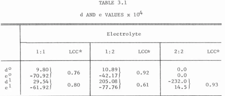
the solution temperature. The values of d and e for 1:1 and 1:2 elec -trolytes, as evaluated from a least-square analysis of the data points

in Figures 3.3 and 3.4, are presented in Table 3.1. The magnitudes of

d and e for 2:2 electrolytes are also presented in this Table. The

evaluation procedure for this last case is discussed later in this

section.

The linear correlation coefficients of the various sets of data suggest that the assumptions which led to the derivation of

equations (3.12) and (3.13) are reasonable. The degree of accuracy of

the proposed model may be sensed in more practical terms by comparing

solu-tions against the experimental ones. Publications on laboratory deter

-minations of the activity and osmotic coefficients of electrolyte

solutions at temperatures other than 25°C are rather scarce and often

incongruent. Literature information on the thermodynamic properties of

sodium chloride solutions at various temperatures is somewhat more

reliable for these properties have been thoroughly studied by several

investigators. The reported experimental activity and osmotic coeffi

-cients of sodium chloride solutions at temperatures between 0°C and

80°C and at concentrations as high as l.Om are listed in Table 3.2.

These two coefficients are calculated in this dissertation by means of

the d and e parameters for 1:1 electrolytes in Table 3.1. The results

of these calculations are presented in Table 3.2.

TABLE 3.1

d AND e VALUES x 104

Electrolyte

1:1 LCC>'< 1:2 LCC* 2:2 LCC>'<

do _9.80}

0.76 10.89} 0.92 0.0

eo _-70.92 -42.17 0.0

dl _{29.54} 205.08}}

0.61 -232.0 } 0.93

el _-61.92 0.80 -77.76 14.5

[image:54.587.82.515.386.570.2]

t,°C

0

25

40

80

TABLE 3.2

TEMPERATURE DEPENDENCE ON THE ACTIVITY AND

COEFFICIENTS OF NaCl SOLUTIONS

I Ycalc

0.1 0.781

0.2 0.735

0.5 0.680

1.0 0.650

0.1 0. 776

0.2

o.

732

0.5 0.679

1.0 0.655

0.1 0.783

0.2 0.727

0.5 0.676

1.0 0.655

0.1 0.755

0.2 0. 710

0.5 0.660

1.0 0.644

aHarned and Owen (1958)

bGibbard et al (1974)

YExp

0.78la

0.731

0.673

0.635

0. 778c

0.735

0.681

0.657

0. 774d 0. 729 0.677 0.658 0.758d 0. 711 0.659 0.640

cRobinson and Stokes (1959)

dEnsor and Anderson (1973)

<Peale 0.932 0.923 0.921 0.935 0.932 0.923 0.921 0.935 0.934 0.922 0.922 0.939 0.926 0.918 0.921

0.964

OSMOTIC ¢Exp 0.933b 0.921 0.911 0.915

0.932c

0.925 0.921 0.936 0.932d 0.924 0.923 0.940 0.927d 0.919 0.918 0.939

The calculated activity coefficients of NaCl in Table 3.2 are

in excellent agreement with the experimental ones over the studied

tern-perature domain. At 80°C a considerable discrepancy between

experi-mental and calculated osmotic coefficients is observed. This

[image:55.583.114.471.155.443.2]

Nonetheless, for the range of temperature of most natural waters, the above assumption yields reasonable results. One may conclude from the results in Table 3.2 that the proposed simplified model may be used with high degree of certainty to compute the thermodynamic properties

of aqueous solutions at temperatures between 0°C and 40°C. At higher temperatures the usage of the model should be discreet .

Harned and Owen (1958) compiled the relative partial molal en -thalpies of dilute divalent cation sulfate solutions at 25°C. These values were used in this dissertation to calculate the Y variables, which correspond to the left side of equation (3.9). TheY variables, as well as their corresponding

x

₁ and

x

₂ values, were computed in the Appendix. It was previously discussed in this section that for most practical cases the last term in equation (3.9) can be ignored. This assumption holds in the following mathematical derivations.

Equation (3.9) is represented by the linear polynomial equation

(3.7). It is initially assumed in this dissertat ion that the b₀ term (i.e.,

a{3

°

/a T), in equation (3. 7) is equal to zero. Ignoring bo, the following relationship is obtained when one divides this equation

(3.14)

If the above assumptions are correct over the studied ionic

strength range, for a given electrolyte solution, a _{plot of Y/X1}

In all cases linearity is preserved for _X2/x1 between 0.04 and 0.27~

This domain of the abscissa corresponds to ionic strengths from 0.36

to 0.026m. Therefore, one may conclude that for this interval the

above assumptions are valid.

The intercept, b1, and the slope of any _{straight line, b 2 , in}

Figure 3.5 correspond to 8~1/8T and8~2/oT respectively. Only two points are plotted for calcium sulfate in Figure 3.5 due to the limited

solubility of gypsum. It is unreasonable to attempt to evaluate b1 and

b₂ for CaS04 from this limited information. _{The b 1} and _{b 2 parameters}

for _Caso4 were predicted according to a procedure described later in this section.

Experimental enthalpy information of concentrated divalent

cation sulfate solutions is extremely limited. The only available

publication on this type of information seems to be the work by Snipes

et al (1975). These researchers have evaluated the relative apparent

molal enthalpies of MgS04 at 40°C and up to 8.0m. The values of Y,

x

_{1 and}

x

2 for these Mgso4 solutions are evaluated in the Appendix.

An attempt is now made to determine the actual magnitude of b₀ for

Mgso

4 solutions. The objective of such a determination is to demon-strate that for most practical cases the net effect of b₀ on the ther-modynamic properties of aqueous solutions is negligible. Subtracting b2X 2 from equation (3.7) yields:

Y - _{b 2}

x

₂

=

b₀

+

b1X1 (3.15)

Graphically calculating _{b 2} from Figure 3.5 one obtains that b2

0.0 0

-.05

-.10

-.15

',

"

.

'Y

:"

·

'

'Y

' _'

•

• MgS04

• ZnS04

A CaS04

• CuS04

'Y

CdS04

.36 .25 .16

_L_L _ I

(mol/kg)

Figure 3.5

'--,

'

"

0.2

'

•

·

,

.

~

,

.

-'

~

·

~

-.,

'

•

'

.

A " .

~'

' _' ' _....

,,""

"-

',

'Y

"

"""

....

.

'

'

·

.09 .04 .0256

- _j

__ L ____ ________ . I ---

then computed from the available information. The results of this computation are plotted as a function of

x

₁ in Figure 3.6. The inte r-cept and slope of the best fit straight line in this figure correspond to b₀ and b1 respectively. The effect of b2 on the value of the depen -dent variable in equation (3.15) may be visualized from the difference between the continuous and the dashed lines in Figure 3.6. The latter line represents a plot of the left side of equation (3.15) ignoring the

contribution of _{b 2} (i.e., b2

=

0.). The following important conclu -sions may be drawn from the graphical results in Figure 3.6:

a) The effects of b2X2 on the left side of equation (3.15) are of importance, especially at low ionic strength. These effects are reflected on the linearity of the full points in Figure 3.6. The excellent linear correlation of such points demonstrates the validity of the proposed magnitude

of _{b 2 •}

b) A least-square analysis of Y

+

b2X2 as a function of

x

₁

shows that b0 and b 1 equal 0.0006/deg and 0.0272/deg. The

assumption that one may neglect the effects of b₀ in dilute solutions is confirmed by the relatively small value of b₀ in comparison with b1. This assumption should yield accurate results up to ionic strengths as high as 2.0 or

3 .Om.

c) The value of _{b 1} calculated from the intercept of Figure 3.5

0.012

0.010

0.008

0.006

0.004

0.002

• Corrected for

{){J

2

/

8

T

o Uncorrected for

ofJ2/

{)T

/

.

7

/

0

/

/

/

/

--

-

-•

/

,

/

/

-

-

0

--o

.

ooo

L---

---

--~L-