Abstract—This paper contributes a numerical method for solving a class of fractional convection diffusion equations with time-space variable coefficients. By implementing Legendre polynomials and also the associated operational matrix, the considered equations will be reduced to the corresponding systems of algebraic equations, which can be solved by computer programming. Also, the error analysis of the suggested method to the exact solutions is provided. Finally, numerical examples are provided to show the efficiency of the presented method.
Index Terms—Legendre polynomials; fractional convection diffusion equations; operational matrix; Sylvester equation; numerical solution
I. INTRODUCTION
RACTIONAL calculus is a field of science and engineering that deals with derivatives and integrals of any arbitrary complex or real order. Since many dynamical systems can be described by fractional-order equation, fractional calculus has drawn the attention of many famous researchers [1-3]. During the last 10 years, with the rapid development of nonlinear science, fractional theory has developed progressively and researchers have found that derivatives and integrals of fractional order are suitable for the description of various physical phenomena such as control, dampling law, acoustic, edge detection, convection diffusion and many other problems [4-8]. Fractional calculus of convection diffusion equations has been widely considered in recent years. Some theoretical works have been done [9,10]. Chang and Nieto [11] proved the existence of solutions for a certain class of fractional differential inclusions with boundary conditions. Stojanovic and Gorenflo [12] proved the existence and the uniqueness of a nonlinear two-term time fractional diffusion wave problem with Cauchy conditions. However, more numerical solutions also are paid attention. Lin et al. [13] applied an explicit finite difference method to investigate stability and convergence of approximation for the variable order nonlinear fractional diffusion equation. Zhuang et al. [14] proposed explicit and implicit Euler
Manuscript received December 7, 2016; revised January 17, 2018. Guo Zhong is with the School of Aeronautic Science and Engineering, Beihang University, Beijing, P.R.China .
Mingxu Yi (Corresponding author) is with the School of Aeronautic Science and Engineering, Beihang University, Beijing, P.R.China (e-mail: [email protected])..
Jun Huang is with the School of Aeronautic Science and Engineering, Beihang University, Beijing, P.R.China.
method for the variable order fractional advection-diffusion equation. Meerschaert et al. [15] applied finite difference method to solve the numerical solution of fractional equation with integrated differential of
t
.In this study, we consider a class of two term time fractional convection diffusion equations with time-space variable coefficients as following:
1 2
1 2
1 2
( , )
( , )
( , )
( , )
( , )
( , )
( , ),
0
1, 0
1
u x t
u x t
t
t
u x t
u x t
c x t
d x t
q x t
x
x
x
t
(1
) with initial and boundary conditions
( , 0)
( ),
u x
f x
(2)(0, )
(1, )
0,
u
t
u
t
( 3) where
1u
t
1and
2u
t
2are fractional derivative of Caputo sense,
u
x
and
u
x
are fractional derivative Riemann-Liouville sense. Here we assume that( , )
q x t
,c x t
( , )
a x v t
( ) ( )
,d x t
( , )
b x v t
( ) ( )
are the known continuous functions,u x t
( , )
is the unknown function,0
1,
2, ,
1 2,
1
,1
2
and1 2
1
.This paper is organized as follows: In section 2, we introduce some necessary definitions and mathematical preliminaries of fractional theory. In section 3, after describing the basic formulation of Legendre polynomials, we give the Legendre polynomials matrix of fractional integration. In section 4, we derive the solute procession of the method. In section 5, we give the error analysis of the method. In section 6, we present several results and discussion to show the efficiency and simplicity of the proposed method. Finally some conclusions are given in section 7.
II. FRACTIONAL CALCULUS
In this section, we introduce some necessary definitions and mathematical preliminaries of fractional calculus theory which are required for establishing our results [1].
Definition 2.1. The Riemann-Liouville fractional integral operator of order
is given byNumerical Method for Solving Fractional
Convection Diffusion Equations with Time-
space Variable Coefficients
Guo Zhong, Mingxu Yi* and Jun Huang
F
IAENG International Journal of Applied Mathematics, 48:1, IJAM_48_1_09
1 0
1
(
)
( )
,
0
( )
(
)( )
( ),
0
t
t
t
u
d
I u t
u t
(4) where
( )
denotes gamma function. And its fractional derivative of order
0
is defined as1 0
( )
, ;
( )( )
1 ( )
, 0 1 .
( ) ( )
n
n
t n t
n n
d u t
n N
dt D u t
d u
d n n
n dt t
(5)
Definition 2.2. The Caputo definition of fractional differential operator is given by
* ( )
1 0
( )
, ;
( )( )
1 ( )
, 0 1 .
( ) ( )
n
n
n t
n
d u t
n N
dt D u t
u
d n n
n t
(6)
The Caputo fractional derivatives of order
is also defined as(
D u t
*)( )
(
I
tnD u t
tn)( )
, the relationship between Riemann-Liouville operator and Caputo operator is given by:
1 ( ) *
0
(
)( )
( )
(0 )
,
!
0,
1
k n
k t
k
t
I D u t
u t
u
k
t
n
n
(7)III. LEGENDRE POLYNOMIALS AND THEIR OPERATIONAL MATRIX OF THE FRACTIONAL INTEGRATION
The shifted Legendre polynomials of order
i
which are defined on the interval [0,1]can be given by [16]1 1
(2
1)(2
1)
( )
( )
( ),
1
1
1, 2,
i i i
i
t
i
P
t
P t
P
t
i
i
i
(8)where
P t
0
( ) 1, ( )
P t
1
2
t
1
. Now, we define( )
2
1 ( )
i i
P t
i
P t
(9) Any functionu t
( )
L
2[0,1)
can be expressed by Legendre polynomials0
( )
i i( )
i
u t
c P t
(10) Ifu t
( )
is piecewise constant and approximated as piecewise constant, Eq.(10) can be rewritten with finite terms, which is0
( )
( )
( )
m
T i i
i
u t
c P t
C
t
(11) wherec
i
u t P t
( ), ( )
i ,[ ,
0,
]
T m
C
c
c
,0
( )
[ ( ),
,
( )]
T mt
P t
P t
.A function
u x t
( , )
L
2([0,1] [0,1])
can be expressed in terms of the Legendre basis. In practice, only the first(
n
1) (
n
1)
term of Legendre polynomials are considered. Hence0 0
( , )
( )
( )
( )
( )
m m
T
ij i j
i j
u x t
a P x P t
x A
t
(12)where
00 01 0
10 11 1
0 1
m
m
m m mm
a
a
a
a
a
a
A
a
a
a
,
( ),
( , ),
( )
ij i j
a
P x
u x t P t
.The operational matrix of integration of a vector
( )
t
is defined as0
( )
( )
t
m
x dx
J
t
(13) For the vector of Legendre basis polynomials, the operational matrixJ
mcan be written as [17]1 1 0 0 0 0
1 1
0 0 0 0
3 3
1
2 1 1
0 0 0 0
2 1 2 1
1
0 0 0 0 0
2 1
m
J
m m
m
(14)
The fractional integration of vector
( )
t
can be approximated as(
I
t
)( )
t
J
m
( )
t
(15) whereJ
mis the Riemann-Liouville fractional operational matrix of integration defined in[16] as[
]
, 1
,
1
m ij m m
J
i j
m
(16) where2
0 0
(2 1)(2 1)
( 1) ( )!( )!
( )! ! ( 1 )( 1)!( !) ( 1)
ij
i k j l j
i
k l
B i j
i k j l
i k k k j l l k
(17)and
1 1
, 1
,
1
ij
B
i ji j
m
(18)IV. METHOD FOR THE NUMERICAL SOLUTION OF THE FRACTIONAL CONVECTION DIFFUSION EQUATIONS WITH
TIME-SPACE VARIABLE COEFFICIENTS
In this part, the Legendre polynomials operational matrix of fractional order is used to solve Eq.(1). We assume that
3 2
( , )
( )
( )
T
u x t
x U
t
x t
(19) where
U
[
u
ij m m]
is an unknown matrix. By integrating Eq.(19) with respect tot
, we get2 2
( , )
( )
( )
( )
T
m
u x t
x UJ
t
f
x
x
(20)IAENG International Journal of Applied Mathematics, 48:1, IJAM_48_1_09
By integrating Eq.(20) with respect to
x
, we obtain0
( , ) ( , )
( ( ))T ( ) ( ) (0)
m m
x
u x t u x t
J x UJ t f x f
x x
(21)
2 0
( , )
(
( ))
( )
( )
( , )
(0)
(0)
T m m xu x t
J
x
UJ
t
f x
u x t
f
xf
x
x
(22)Combining Eq.(15), Eq.(20) and Eq.(21), we have
2 2
( , )
(
m( ))
T m( )
x( )
u x t
J
x
UJ
t
I
f
x
x
(23)1 1 1 0
( , )
(
( ))
( )
( , )
( )
(0)
(2
)
T
m m m
x
x
u x t
J J
x
UJ
t
x
x
u x t
I
f x
f
x
(24)By integrating the Eq.(21) with respect to
x
from 0 to 1, we obtain0
(1, )
(0, )
(
)
( )
(1)
( , )
(0)
(0)
T
m m
x
u
t
u
t
J L UJ
t
f
u x t
f
f
x
(25)where
L
[ , ,
l l
0 1, ]
l
m T, and2 0
2
1
(
)!
( 1)
1
(
)!( !)
i
i k i
k
i
i
k
l
i
i
k
k
.Substituting Eq.(3) and Eq.(25) into Eq.(24), we have
1 1
1
( , )
(
( ))
( )
( )
(
)
( )
(1)
(0)
(2
)
T
m m m x
T
m m
u x t
J J
x
UJ
t
I
f x
x
x
J L UJ
t
f
f
(26)Similarly, by integrating Eq.(19) with respect to
x
twice, we get
22
0
( , )
( ) T ( ) (0, )
m
x
u x t u
J x U t x u t
t x t
(27)
Then we have
22 1 1
0
1
0
( , )
( ) T ( )
m m t
x
t x
u x t u
J x UJ t xI
t x t
u I t (28)
where
1or
2. The value of2 0
x
u
x t
is calculated as2
1 0
0
(
m)
T( )
x x
x
u
u
u
J L U
t
x t
t
t
(29)Substituting Eq.(3) and Eq.(29) into Eq.(28), we have
2
11
( , )
( )
( )
(
)
( )
T m m T m mu x t
J
x
UJ
t
t
x J L UJ
t
(30) Let 1 1 2( , )
( , )
( ) ( )
( )
( (1)
(0))
( ) ( )
( ) ( )
( )
(2
)
x
x
g x t
q x t
a x v t I
f x
x
f
f
a x v t
b x v t I
f
x
.Substituting Eq.(23), Eq.(26), Eq.(30) into Eq.(1), we have
1 2 1 1 2 1 2 1 1 1 ( ( )) ( ) ( ) ( ) ( )( ( )) ( ) ( )( ( )) (2 ) ( ) ( ) ( , ) T T
m m m m T
T m T
m m m
m
J x x J L U J J t
x J L
a x J J x a x b x J x
UJ t v t g x t
(31)
Dispersing Eq.(31) by the points
(
0.5) /
s s
x
t
s
m
,s
0,1, 2,
,
m
1
, the coefficientsa x
( )
,b x
( )
,v t
( )
andx
can be transferred into some diagonal matrices asA V B X
, , ,
, respectively, such as 0 1 10
0
0
0
0
0
ma
a
A
a
.The function
g x t
( , )
is also transferred into[ ( , )]
i j m mG
g x t
. Then Eq.(31) can be transformed into a Sylvester equation which is solved by computer software. Using Eq.(22), we can acquire the approximation ofu x t
( , )
.V. ERROR ANALYSIS
Suppose that
( , )
x t
is a bivariate polynomial that interpolateu x t
( , )
at points( , )
x t
i j that defined in Eq.(12), we conclude that [18]1 1 1 1
1 1 1 1
2 2 1 1
1 1 2 1 1
( , )
( , )
( , )
( , )
(
)
(
)
(
1)!
(
1)!
( ,
)
(
)
(
)
((
1)!)
m m m m
i j
m i m j
m m m
i j
m m i j
u x t
x t
u
t
u x
x
x
t
t
x
m
t
m
u
x
x
t
t
x
t
m
(32)where
,
,
and
are in [0,1]. Let [0,1] [0,1] and
1 1 2 2
1 1 1 1
( , ) ( , ) ( , )
( , ) ( , ) ( , )
max max , max , max
m m m
m m m m
x t x t x t
u x t u x t u x t M
x t x t
, then we have
2
1
( , )
( , )
2
2 (
m1)!
2 (
1)!
M
u x t
x t
m
m
(33)Theorem 1. Let
u x t
( , )
be a sufficiently smooth function on2
[0,1]
L
that approximated by Legendre polynomial as( , )
( )
( )
u x t
x A
t
, then an upper bound to estimate the error is as2
1
( , ) ( ) ( ) 2
2 (m 1)! 2 ( 1)!
E
M
u x t x A t
m m
(34)
Proof.
( , )
x t
, we can get[16]IAENG International Journal of Applied Mathematics, 48:1, IJAM_48_1_09
( , )
( )
( )
( , )
( , )
E E
u x t
x A
t
u x t
x t
(35) Then we have2
1 1 2
0 0
1 1 2
0 0
( , ) ( ) ( )
( , ) ( ) ( )
( , ) ( , ) E
u x t x A t
u x t x A t dxdt
u x t
x t dxdt
(36)
Using Eq.(33), we can obtain
2
2 1 1
2 0 0
2
2
( , ) ( ) ( )
1 2
2 ( 1)! 2 ( 1)!
1 2
2 ( 1)! 2 ( 1)!
E
m
m
u x t x A t
M
dxdt
m m
M
m m
(37)Therefore
2
1
( , ) ( ) ( ) 2
2 (m 1)! 2 ( 1)!
E
M
u x t x A t
m m
.
This completes the proof.
VI. NUMERICAL EXAMPLE
Example 1: Consider the following space time fractional convection-diffusion equation [19]
( , )
( , )
( , )
( )
( )
( , ),
0
1,
0
1
u x t
u x t
u x t
b x
a x
q x t
t
x
x
x
t
,
2
( , 0)
(1
),
0
1
(0, )
(1, )
0,
0
u x
x
x
x
u
t
u
t
t
,where
a x
( )
(2.8) / 2
x
,b x
( )
x
0.8 ,2 1.2 1.8 2
( , )
2
(1
)
/ (2.2) 0.2
(1
)
q x t
x
x t
x
t
, theexact solution is
u x t
( , )
x
2(1
x
)(1
t
2)
when0.8
,
1.5
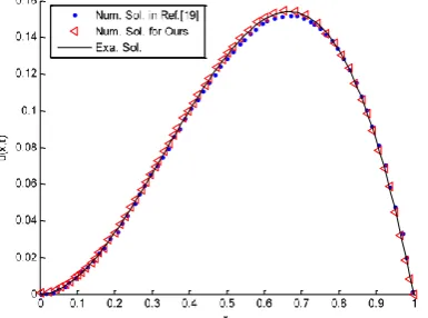
.The comparison between the numerical solutions and the exact solution by Legendre polynomials method (LPM,
0.2
t
,m
3
) and Haar wavelets method (HWM,ˆ
64
m
) are shown in Fig.1. [image:4.595.44.291.52.495.2]Fig. 1. The comparison between Num. sol. and Exa. Sol. of HWM and LPM.
Table I
The absolute errors for t0.2and different
m
,m
ˆ
.x
m
ˆ 16
m
2
m
ˆ 32
m
3
HWM LPM HWM LPM
0.1 4.6e-003 3.5e-008 1.0e-004 1.4e-008 0.2 2.6e-003 4.1e-008 2.6e-003 3.1e-008 0.3 1.6e-002 6.0e-007 6.0e-003 7.9e-008 0.4 8.9e-003 6.8e-006 8.8e-003 9.0e-007 0.5 1.6e-003 5.3e-006 1.5e-003 4.5e-007 0.6 7.6e-003 6.3e-008 2.8e-003 2.4e-006 0.7 3.6e-003 7.2e-007 1.5e-003 8.1e-008 0.8 1.1e-002 9.4e-008 4.8e-003 8.9e-009 0.9 1.6e-002 1.0e-005 1.6e-002 1.7e-007
We have calculated the absolute errors by using our method and Haar wavelets method and tabulated the results in the Table I. Through Table I, we can also see that the errors are smaller and smaller when
m
andm
ˆ
increase, and the errors based on our method are less than the errors in Ref.[19].From the comparison between two methods for the first example, we conclude that Legendre polynomials method is more accurate when solving the same equations.
Example 2: Consider Eq.(1) and choose
1
2
0.5
,1
0.8
,
2
0.5
,
0.9
,
1.8
and0.9 1.8
( )
(3.1)
, ( )
(2.2)
, ( )
a x
x
b x
x
v t
t
, the function2 0.2 2 0.5
( , )
(1
)
/ (1.2)
(1
)
/ (1.5) 2.07 (1
)
q x t
x
x t
x
x t
xt
t
and
f x
( )
x
(1
x
2)
. The exact solution of the problem is2
( , )
(1
)(1
)
[image:4.595.74.267.593.736.2]u x t
x
x
t
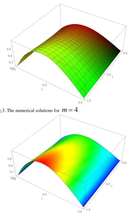
. We applied the Legendre polynomials method to solve this problem for various values ofm
. The numerical solutions form
3, 4
and the exact solution are shown in Fig. 2, Fig.3 and Fig. 4.Fig.2. The numerical solutions for
m
3
.IAENG International Journal of Applied Mathematics, 48:1, IJAM_48_1_09
Fig.3. The numerical solutions for
m
4
.Fig.4. The exact solution.
[image:5.595.55.355.49.643.2]The absolute errors between the exact solution and the numerical solution are displayed as follows:
Fig. 5. The absolute error for Example 2 of
m
3
.From Fig. 2-4, we can see clearly that the numerical solutions are very good agreement with the exact solution. It can be also seen that the proposed method is very efficient and accurate for solution of this problem. From Fig. 5, we can find that the absolute errors are very tiny and only a small number of Legendre polynomials are needed when
n
3
.VII. CONCLUSION
In this paper, the authors have proposed a numerical algorithm based on Legendre polynomials operational matrix to solve a class of two term time fractional convection-diffusion equations with initial condition. The Legendre polynomials operational matrix of fractional
integration has been used for transforming the time fractional convection-diffusion equation into a Sylvester equation that can be solved easily. The error analysis of the method has been shown in section 5. The accuracy of the proposed method is shown for numerical examples.
REFERENCES
[1] Y.L. Li, W.W. Zhao, “Haar wavelet operational matrix of fractional order integration and its applications in solving the fractional order differential equations,” Appl. Math. Comput., vol. 216, pp. 2276-2285, 2010.
[2] H. Sun, W. Chen, C. Li et al, “Fractional differential models for anomalous diffusion,” Physica A-Statistical Mechanics and its Applications, vol.389, no.14, pp. 2719-2724, 2010.
[3] H. Song, M.X. Yi, J. Huang, Y.L. Pan, “Numerical solution of fractional partial differential equations by using Legendre wavelets,”
Engineering Letter, vol. 24, no. 3 pp. 358-364, 2016.
[4] M. Ichise, Y. Nagayanagi, T. Kojima, “An analog simulation of noninteger order transfer functions for analysis of electrode process,”
Journal of Electroanalytical Chemistry,vol. 33, pp. 253- 265, 1971. [5] Z.M. Yan, F.X. Lu, “Existence of a new class of impulsive Riemann-
Liouville fractional partial neutral functional differential equations with infinite delay,” IAENG International Journal of Applied Mathematics, vol. 45, no. 4, pp.300-312, 2015.
[6] O. Heaviside, Electromagnetic Theory, Chelsea, New York, 1971. [7] H. Song, M.X. Yi, J. Huang, Y.L. Pan, “Bernstein polynomials method
for a class of generalized variable order fractional differential equations,” IAENG International Journal of Applied Mathematics, vol. 46, no.4, pp.437-444, 2016.
[8] V.V. Anh, J.M. Angulo, M.D. Ruiz-Medina, “Diffusion on multifractals,” Nonlinear Analysis, vol.63, pp. e2053-e2056, 2005. [9] W. Chen, “A speculative study of 2/3-order fractional Laplacian
modeling of turbulence: Some thoughts and conjectures,” Chaos, vol.16, 023126, 2006.
[10] Asgari M, “Numerical Solution for Solving a System of Fractional Integro-differential Equations,” IAENG International Journal of Applied Mathematics, vol. 45, no. 2, pp.85-91, 2015.
[11] Y.K. Chang, J.J. Nieto, “Some new existence results for fractional differential inclusions with boundary conditions,” Math. Comput. Model., vol.49, pp. 605-609, 2009.
[12] M. Stojanovic, R. Gorenflo, “Nonlinear two term time fractional diffusion-wave problem,” Nonlinear Anal-real., vol.11, pp. 3512- 3523, 2010.
[13] R.Lin, F. Liu, V. Anh, I. Turner, “Stability and convergence of a new explicit finite-difference approximation for the variable-order nonlinear fractional diffusion equation,” Appl. Math. Comput., vol.212, pp.435-445, 2009.
[14] P. Zhuang, F. Liu, V. Anh, I. Turner, “Numerical methods for the variable-order fractional advection-diffusion equation with a nonlinear source term,” SIAM J. Numer. Anal., vol.47, pp. 1760- 1781, 2009. [15] M.M. Meerschaert, C. Tadjeran, “Finite difference approximations for
fractional advection- dispersion flow equations,” J. Comput. App. Math., vol.172, no.1, pp. 64-77, 2004.
[16] A. Lotfo, M. Dehghan, S.A. Yousefi. “A numerical technique for solving fractional optimal control problem,” Comput. Math. Appl., vol.62, pp. 1055-1067, 2011.
[17] R.Y. Chang, M.L. Wang, “Shifted Legendre direct method for variational problems,” J. Optim. Theory. Appl., vol.39, pp. 299-307, 1983.
[18] M. Gasca, T. Sauer, “On the history of multivariate polynomial interpolation,” J. Comput. Appl. Math., vol. 122, pp. 23-35, 2001. [19] Y.M. Chen, Y.B. Wu, et.al., “Wavelet method for a class of fractional
convection-diffusion equation with variable coefficients,” Journal of Computational Science, vol.1 pp.146-149, 2010.