Abstract—Participants were given sheets printed with signals of sine waves ranging from a single wave to ones having higher frequencies added. The signals were digitized to give data points at a number of sampling rates, the lowest at the Nyquist-Shannon frequency and up three times that frequency. At sampling rates less than the Nyquist-Shannon frequency, a machine is unable to accurately reconstruct a signal. Hence the aim was to determine a person’s ability to reconstruct signals at sampling rates at and higher than the Nyquist-Shannon frequency. Data showed that the RMS error decreased with signal bandwidth and also with sampling rate. At high sampling rates, participants were able to accurately reconstruct the signal, although this was not consistent across participants. At low sampling rates and low bandwidth, there was a tendency to include frequencies in the estimated signal that were not in the actual signal.
Index Terms—Signal reconstruction, Nyquist criterion, signal bandwidth, sampling rate
I. INTRODUCTION
EOPLE are often presented with information that is in a digital form, due to the way in which the information is gathered or can be conveniently presented. This may be, for example, the trends in cost of housing, the weather as dependent on month of the year, the performance of the stock exchange and so on. In order to make a reasonably accurate estimate of the numerical value at a certain part of the digital information, it may be necessary to convert the digital data into an analogue form. For instance, a travel guide may give the temperature in parts of the UK on a monthly basis. The traveler can plot the data and estimate the analogue form and consequently obtain an approximate temperature for the time at which they will be visiting that country. The question posed by this study is “how accurately can a person reconstruct the analogue information based on the detail in the digital form of the information?”
It is well known that, under special circumstances, a digital signal may be reconstructed by computer to its analog form without error, that is, all frequency components and amplitudes may be found from the digital signal. The circumstances under which this reconstruction may be achieved by machine is given by the Nyquist-Shannon
Manuscript was submitted on 26 December, 2017.
1Dept. of Systems Eng. and Eng. Management, City University of Hong
Kong, Kowloon Tong, Hong Kong. (email: [email protected])
2Dept. of Logistics Management, School of Business, North Minzu
University, Yinchuan, Ningxia, China.
3Dept. of Mechanical Engineering, University of Melbourne, Melbourne
3010, Australia.
sampling theorem. This theorem states that “If a function x(t) contains no frequencies higher than B Hz, it is completely determined by giving its ordinates at a series of points spaced 1/(2B) seconds apart… A sufficient sample-rate is therefore 2B samples/second, or anything larger. Equivalently, for a given sample rate fs, perfect reconstruction is guaranteed possible for a bandlimit B < fs/2” [1]. When the sampling rate is less than the Nyquist-Shannon sampling rate aliasing may occur, so that it is not possible to differentiate the various frequencies within a signal.
Thus, for accurate machine reconstruction of a signal, it is necessary to have a sampling rate that is at least twice the highest frequency occurring in the signal. More recently, it has been shown that, under special circumstances, it is possible to have somewhat lower sampling rates and still recover the full details of a signal [2,3].
What is not known is if a human can accurately reconstruct an analogue signal when given the discrete digital values on a graph. Can the correct frequency content be recovered along with the amplitudes of the components of the original analogue signal? What conditions are necessary for this reconstruction in terms of the sampling rate and the associated bandwidth of the analog signal?
It was the aim of our experiments to present people with simple signals that are digitized at different rates and which have different bandwidths and to determine how human performance compares with that of machine signal recovery. It is noted that, when the sampling rate is higher than the Nyquist-Shannon sampling rate, a machine can perform the task exactly, that is, the machine can determine both the frequency components and amplitudes exactly as in the original analog signal. As far as the authors are aware, no such tests of human performance have been reported.
II. METHOD
A. Participants
Thirty self-reported healthy male college students participated in this study. Ages of the subjects ranged between 18 and 25, having a mean and median of 20.97 and 20.5 years. All participants were fully informed of the purpose of the experiment, and their written consent to participate was taken.
B. Signals and Sampling Rates Used in the Experiment
In this preliminary study of signal reconstruction by humans, we selected simple signals in which the bandwidth was a multiple of the basic bandwidth. We used sine waves
Human Reconstruction of
Digitized Graphical Signals
Coskun DIZMEN1,2, and Errol R. HOFFMANN3
and summed sine waves as the signals for the study. Signals used in the experiment are listed in Table 1. Sampling rates are expressed in terms of the Nyquist Period of each signal and therefore the numerical values of sampling rates for each of the signals were different (Table 2). Note that we used the minimum sampling rate as that of the Nyquist value – this value can introduce considerable uncertainty into the reconstruction process due to the problem of aliasing. We introduced this value of sampling in order to determine if humans had any problem in reconstructing the signal, in the same way as a machine might have.
TABLE I
THE FOUR GRAPHICAL SIGNALS USED IN THIS EXPERIMENT.
Signal
Highest Frequency
[B]
Nyquist Period [1/(2B)]
sin(t) 1/(2pi) pi/1
sin(t) + sin(2t) 2/(2pi) pi/2
sin(t) + sin(2t) + sin(3t) 3/(2pi) pi/3
sin(t) + sin(2t) + sin(3t) + sin(4t) 4/(2pi) pi/4
Signals are a simple summation of sine waves.
TABLE II
NUMERICAL VALUES OF THE SAMPLING PERIODS FOR EACH OF THE FOUR SIGNALS IN TERMS OF THE NYQUIST PERIOD AND THE HIGHER SAMPLING
RATES OF 1.5, 2.0, 2.5 AND 3.0 TIMES THE NYQUIST FREQUENCY.
a The horizontal distance between two consecutive points in the discrete
signal.
C. Procedure
In order for participants to become familiarized with the experimental task, subjects were shown analog and digitized versions of two representative signals (i.e. sin(t) and sin(t)+sin(2t)+sin(3t)+sin(4t)+sin(5t)) before the experimental trials were run.
Although all participants had basic knowledge of mathematical functions, none had studied the Nyquist-Shannon Theory before they took part in the experiment. Participants were instructed to connect the dots with a pen to reconstruct a smooth curve which should be a continuous function without any sharp corners.
All of the signals were digitized on paper, over 2π region, covering one full cycle of the signal. Digitization was based on Tables 1 and 2; and, as all signals used in this experiment were periodic with a period of 2π, the beginning and ending points of a signal had exactly the same ordinates. The starting and ending points of the signal were also labeled on the paper. Each subject attempted to reconstruct each signal one and only one time. Since showing the same signal more than once would cause a learning effect, each subject was assigned a sampling rate and observed all signals with the
same specific sampling rate once only. Therefore, in total, each subject was given 4 separate sheets (one signal per page). Samples of the digitized signals, in the random order given to participant 30 are shown in Figure 1. These are for the highest sampling rate 5 and for each of the signals 1 to 4.
D. Data Analysis
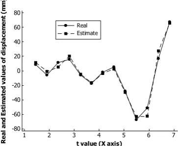
For data analysis, 13 sample points were taken from each paper. The error, i.e. the difference between the actual analog signal and the one reconstructed by the subject was measured. Errors were standardized by dividing them with the amplitude of the actual analog signals, which differed for each presented signal. Root-mean-square (RMS) of the standardized errors were then calculated and used in the following analysis. Sample estimated waves for Signals 1 and 3 are shown in Figures 2 and 3 to illustrate the form of errors that occurred at different signal bandwidth and sampling rates.
III. RESULTS
Data are shown in Figure 4 for the mean values of RMS error as a function of the sampling rate and the bandwidth of the signals. Anova of the RMS data, using a mixed model with participants random and nested under the sampling rate variable, gave main effects of Sampling Rate [F(4,25) = 12.72, p<.001, 2.67
p
] and Signal [F(3,75) = 16.29,
p<.001, 2.39 p
]. There was also a significant interaction between these factors [F(12,75) = 2.22, p<.05, 2.26
p
].
Post-hoc tests using the Tukey HSD procedure showed that, for sampling rate 1, signal 4 had significantly lower RMS than other 1 and 2 (p<.01) and less than 3 (p<.05). Also Signal 1 had greater RMS than 4 and 3 (p<.01) and 2 (p<.05). At sampling rate 2, Signal RMS than all other Signals (p<.01). Sampling rates 3 , 4 and 5 showed no significant differences between signals.
Estimated signals
In order to test whether the estimated signals corresponded to the actual signals, a number of tests were performed:
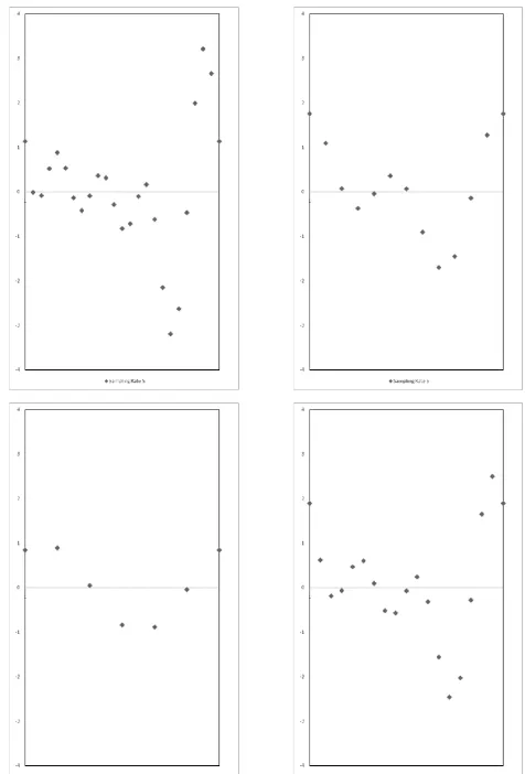
(i) A range of frequencies were regressed to the estimated data to determine the approximate frequency content of the estimated signals. These frequencies were .25, .5, 1, 2, 3, 4, 5 and 6 Hz. Initially, a stepwise regression was made in terms of the 13 digitized values of ordinates of the estimated signal with the eight frequencies. The significant values were then regressed to determine the significance level of each term and the confidence intervals associated with the constant term and coefficients of the frequency terms in the regression. Table 3 lists the significant terms. The right-hand column in this table, lists the number (out of six regressions) that showed constants that were encompassed by the zero value, ± confidence interval, and also the coefficients that had confidence intervals encompassing the value of unity. Figure 5 illustrates the number of estimated signals that satisfied the criteria for an acceptable fit to the actual signals (ii) Injected frequencies. These are the
Numeric Value of Sampling Period
Sampling
Rate Sampling Period
a Signal
1
Signal 2
Signal 3
Signal 4
SR1 NyquistPeriod 3.142 1.571 1.047 0.785
SR2 NyquistPeriod/1.5 2.094 1.047 0.698 0.524
SR3 NyquistPeriod/2 1.571 0.785 0.524 0.393
SR4 NyquistPeriod/2.5 1.257 0.628 0.419 0.314
frequencies that were significant in the regressed estimated signals that were not in the actual signals. The sum of these for the different signals as a function of the sampling rate is shown in Figure 6. Note that there is a gap in these distributions at the frequency of the actual signal frequencies, as any significant term was then not an injected frequency. 7 6 5 4 3 2 1 30 20 10 0 -10 -20 -30 -40
t value (X axis)
[image:4.595.312.542.60.210.2]R ea l a nd e st im at ed d is pl ac em en t (m m ) Real Estimate
Fig. 2. Sample plot of real and estimated signals of a single participant for Signal 1 with a sampling rate of three times the Nyquist frequency.
7 6 5 4 3 2 1 80 60 40 20 0 -20 -40 -60 -80
t value (X axis)
[image:4.595.54.236.351.500.2]R ea l a nd E st im at ed v al ue s of d is pl ac em en t (m m ) Real Estimate
Fig. 3. Sample plot of real and estimated signals of a single participant for Signal 3 with a sampling rate of three times the Nyquist frequency.
5 4 3 2 1 0.4 0.3 0.2 0.1 0.0 Sampling Rate A ve ra ge n or m al iz ed R M S e rr or ( m m ) Signal 1 Signal 2 Signal 3 Signal 4
Fig. 4. Average normalized RMS error as a function of sampling rate and the four signals of increasing bandwidth.
Signal SR 4 3 2 1 5 4 3 2 1 5 4 3 2 1 5 4 3 2 1 5 4 3 2 1 6 5 4 3 2 1 0 N um be r w it h co ef fi ci en ts w it hi n + C I
Fig. 5. Accuracy of estimated signals. These are the number of estimates that had a constant with a value within zero +/- CI and coefficients of terms with value within unity +/- CI. SR = sampling rate.
TABLE III
DATA FOR SIX PARTICIPANTS FOR EACH SIGNAL 1 TO 4 SHOWING THE FREQUENCY CONTENT OF THE ESTIMATED SIGNALS.
Signal SR Constant .25 .5 1 2 3 4 5 6 #OK
1 1 1 5 4 5 4 1 1
1 2 1 1 5 5 1 0
1 3 4 2 6 1 4
1 4 2 2 6 2 2 1 2
1 5 6 2 6 1 0
2 1 3 1 5 5 1 2 3
2 2 3 6 6 2 2 3
2 3 6 6 6 2
2 4 5 6 6 1 1 5
2 5 6 6 6 1 6
3 1 3 6 6 5 2 2 3
3 2 2 6 6 6 2 1 4 2
3 3 1 6 6 6 2 1 3
3 4 3 6 6 6 1 3
3 5 5 6 6 6 1 5
4 1 4 2 4 6 6 6 4
4 2 5 6 6 6 6 1 5
4 3 6 6 6 6 6 6
4 4 6 6 6 6 6 6
4 5 6 6 6 6 6 6
Sampling Rates of ‘1’= Nyquist frequency; ‘2’ = 1.5 x Nyquist frequency etc, up to 3 x Nyquist frequency, in steps of .5. Signal 1 is a pure sine wave having only frequency 1; Signal 2 is the sum of two sine waves (double bandwidth) up to Signal 4 being the sum of four sine waves (three times the bandwidth of Signal 1).
‘Constant’. In all cases the actual value was zero. The column indicates the number of participants having CI encompassing a zero value.
Numbers .25, .5 ---- 6. Indicates the number of participants having significant contributions of this frequency component and with the CI of the coefficient encompassing the value of unity.
[image:4.595.55.279.553.721.2]IV. DISCUSSION
A. Effects of Bandwidth and Sampling Rate
Somewhat counter-intuitively, the estimated signals were closer to the actual signals at the higher bandwidths. This arose from the higher frequency of sampling associated with the higher Nyquist-Shannon frequency. Thus, with more data points to guide them, participants were better able to estimate the actual signal. This is clearly shown in Figures 4 and 5. Here it is shown that the RMS error of the estimated signal decreases rapidly with both the sampling rate and the signal bandwidth, so that at the highest value of each of these factors, almost all estimates were within the confidence intervals of both the constant and coefficients relating the estimated and actual signal coordinates. There are some non-uniformities in the curves shown in Figure 4; these likely arose from the fact that different participant groups were used for each of the sampling rates.
B. Low Bandwidths
Another important result is that participants appeared to have most difficulty in constructing signals at low bandwidths, and it was here that they injected more high and low frequencies into the estimated signals than were in the actual signals (Figure 6). As noted earlier, reconstruction of a signal at this lowest of sampling rates can introduce problems due to aliasing of the signal. Figure 6 clearly shows the effect in that the injected or introduced frequency components are large in number. This is an effect that might be expected with signal aliasing, where it is possible for both lower and higher frequency components to be introduced.
C. Further Experiments Required
The present experiments were for a simple addition of
sine waves. Further work could include the effects of different wave forms and also on phase differences between the component waves.
D. Practical Implications of the Results
There are occasions when it is necessary to study trends, such as annual changes in a variable, when the available data is say in a monthly or quarterly form. In those circumstances, it is necessary to estimate from curves interpolated between data points to obtain the relationship between the variable and the time at which the data were collected. The data of this experiment will give an indication of the necessary density of data points for obtaining a reasonably accurate estimate of such quantities.
V. CONCLUSION
These preliminary experiments indicate that people can make a reasonable estimate when reconstructing a digital signal to arrive at the original analogue signal. The accuracy of the estimates is strongly dependent both on the bandwidth of the signal and the period of digitizing of the signal.
REFERENCES
[1] Shannon, C.E. 1998. Communication in the presence of noise. Proceedings IRE, 86(2), 447-457.
[2] Hamill, Joseph; Caldwell, Graham E.; Derrick, Timothy R., 1997. Reconstructing Digital Signals Using Shannon's Sampling Theorem. Journal of Applied
Biomechanics, 13 (2), 226-238.
[3] Petrellis, N., 2014. Undersamples information recovery in OFDM environment. International Journal of Latest
Research in Science and Technology, 3(3), 40-46.
Band Width Injected Frequency
4
3
2
1 6.
00
5.
00
4.
00
3.
00
2.
00
1.
00
0.
50
0.
25
6.
00
5.
00
4.
00
3.
00
2.
00
1.
00
0.
50
0.
25
6.
00
5.
00
4.
00
3.
00
2.
00
1.
00
0.
50
0.
25
6.
00
5.
00
4.
00
3.
00
2.
00
1.
00
0.
50
0.
25
14
12
10
8
6
4
2
0
N
um
be
r
of
o
cc
ur
re
nc
es
o
f
in
je
ct
ed
f
re
qu
en
[image:5.595.121.473.513.750.2]cy