Direct numerical simulation of a decelerated wall bounded turbulent shear flow

DOI: 10.1017/S0022112003005883 Printed in the United Kingdom

Direct numerical simulation of a decelerated

wall-bounded turbulent shear flow

By G. N. C O L E M A N1, J. K I M2 A N D P. R. S P A L A R T3

1_{School of Engineering Sciences, University of Southampton, Highfield Campus,}

Southampton, SO17 1BJ, UK

2_{Mechanical and Aerospace Engineering, University of California, Los Angeles, CA 90095, USA}

3_{Boeing Commercial Airplanes, Seattle, WA 98124, USA}

(Received24 July 2002 and in revised form 2 June 2003)

A fully developed turbulent channel flow is subjected to a mean strain that approxi-mates that in a spatially developing adverse-pressure-gradient (APG) boundary layer. This is done by applying uniform irrotational temporal deformations to the flow domain of a conventional direct numerical simulation channel code. The velocity difference between the inner and outer layer is also controlled by accelerating the walls in the streamwise plane, in order to duplicate the defining features of both the inner and outer regions of an APG boundary layer. Eventually, the flow reverses at the wall. We address basic physics and modelling issues, and create a database that makes detailed testing of turbulence models easy. As in the corresponding spatial layers, distinct inner- and outer-layer dynamics are observed: a decrease in turbulence intensity near the wall is accompanied by increased energy in the outer layer. The ‘extra strain’ effect associated with the diverging outer-layer streamlines is documented, particularly in the Reynolds-stress budgets.

1. Introduction

behaviour of the mean statistics (rather than the instantaneous coherent structures), and attempt to extract implications for modelling non-trivial flows.

One of the motivations for this work is the need to understand and model the distinct ways in which near-wall and outer-layer turbulence respond to an APG. A classical result of subjecting a boundary layer, laminar or turbulent, to an APG is reduction of the near-wall shear. This inner-layer effect leads to reduced production of turbulence kinetic energy (Nagano, Tsuji & Houra 1997). The outer-layer dynamics are less certain. Some have proposed that a sudden change in streamwise pressure gradient dP /dx does not affect the outer layer until the surface reduction in mean shear ∂U/∂y propagates sufficiently far from the wall (Smits & Wood 1985). Until this happens, it is assumed that turbulence convecting along an outer-layer streamline is unaltered by streamwise changes of dP /dx. In support of this view is the fact that, to within the linear (i.e. weak-turbulence) inviscid idealization, ∂U/∂y remains constant along a mean streamline – which suggests that the outer-layer turbulence is affected by APG perturbations only indirectly, through viscous (and turbulent) diffusion of changes they induce at the surface. However, the APG might have another, more direct, outer-layer effect through the strain rate components associated with the divergence of the mean streamlines. Although the magnitude of these ‘extra’ strains – the mean streamwise compression ∂U/∂x < 0 and wall-normal stretching

∂V /∂y >0 – is typically much weaker than the mean shear is in the more active region of the boundary layer, they become non-negligible at face value in the outer layer, where∂U/∂y→0. Since even a slight distortion or reorientation of eddies away from the shape they obtain after coming into equilibrium with a slowly varying∂U/∂ycan have profound dynamic consequences (Townsend 1961; Bradshaw 1973, 1987, 1988; Hanjali´c & Launder 1980; Smits & Wood 1985), it is conceivable that either or both of the APG strains∂U/∂x <0 and∂V /∂y >0 might produce significant outer-layer alterations, unrelated to those that diffuse from the near-wall region. Many of our results will be shown after a total strain of 0.365 which means that a material line that was initially at 45◦ to the wall, leaning downstream as in many models of the outer-layer coherent structures, ends up at 64◦ (i.e. arctan[exp(0.365)/exp(−0.365)]) to the wall.

We examine the outer-layer effects of an APG by studying a time-developing idealization of a spatially developing APG boundary layer, using DNS. The time-developing flow allows a better statistical sample, which is essential for the budgets, and a higher Reynolds number than a DNS of a spatial APG flow such as that of Spalart & Watmuff (1993). As an idealization, the strained channel cannot be expected to provide the final word on this subject; it should, however, given the basic features shared with the spatial boundary layer, make a meaningful contribution to the topic. Another motivation for what follows is to publicize the strained-channel flow as a candidate for future turbulence model testing and development.

In the next section, we introduce and motivate the strained-channel approach, here for the case of a two-dimensional mean flow. Histories of Reynolds-stress statistics and budgets from the DNS, and a discussion of their implications, are then presented. The final section contains a summary of the work and general conclusions regarding the physics and modelling of non-equilibrium APG boundary layers.

2. Approach

Fluid element

U U

x y

Streamlines U x

y

Channel walls

t = 0

t > 0 (b)

(a)

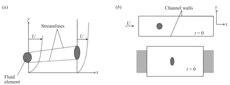
Figure 1.Side view of two-dimensional APG boundary layer. (a) Spatially developing flow.

(b) Initial and deformed domain of time-developing strained-channel idealization.

domain (including the walls) of an initially fully developed incompressible channel flow (figure 1b). The in-plane wall motion duplicates the bulk deceleration of the APG (leading to a reduction in the wall shear stress), by causing the difference between the mean centreline velocity uc and wall velocity uw to decrease at an appropriate

rate (see below). It is equivalent to controlling the Poiseuille pressure gradient. The imposed strain, on the other hand, supplies the irrotational deformation (streamwise compression with wall-normal divergence) associated with the APG. Solutions are obtained using DNS, which resolves all relevant scales of motion so that no turbulence or subgrid-scale model is needed.

The approach to the strain is similar to that of Rogallo (1981), except that instead of distorting spatially homogeneous turbulence u(x, t), here the flow u(x, t) is between two no-slip surfaces and will contain both fluctuations u(x, t) and an inhomogeneous mean u(y, t). (Rogers (2002) has also performed a homogeneous-strain/inhomogeneous-flow DNS, but for a free shear flow, free of no-slip boundaries.) This strategy is based on the observation that the essential perturbation felt by the outer region of an APG boundary layer is not the pressure gradient as such, which has no effect on vorticity, but the ∂U/∂x =−∂V /∂y <0 mean strain that it causes. We use a three-dimensional flow domain that is spatially periodic in the streamwisexand spanwisez directions and has two no-slip ‘elastic’ plane walls, and thus approximate the spatially developing problem with a temporally evolving one. Away from the walls, the channel turbulence is subjected to mean-flow variations in time that correspond to convective changes in a boundary layer (figure 1). The behaviour of the very-near-wall turbulence will also be relevant to the boundary layer, provided the magnitude of the wall shear remains much larger than the applied rate of strain (which, as is shown below, will be true here until just before the skin friction changes sign). The essential characteristics of spatially developing pressure-driven shear layers are thereby captured in a wall-bounded flow that maintains its streamwise and spanwise homogeneity, with great benefits to numerical and statistical efficiency. When averages are discussed we use U and u, respectively, to denote the imposed deformations and the temporally evolving profiles in the channel (averaging the latter over the directions parallel to the walls). An indication of the validity of this approach is verification that the outer-layer mean velocity profiles evolve appropriately (see figure 4).

The imposed deformation field Ui varies linearly in space according to Ui(x, t) =

Aij(t)xj, where each component of the spatially uniform velocity gradient Aij is

associated with the applied strainAij is also constant in time, but linear in space (see

equation (2.8) of CKS). In contrast, since during the straining the velocity fieldu(x, t) remains homogeneous inx andz(and the flow is incompressible), so does the actual pressure p(x, t) in the channel, i.e. the pressure fluctuations† remain periodic in x

andz, and the mean gradient dp/dx= 0. (The externally imposed uniform pressure-gradient/body-force, which drove the Poiseuille flow before the strain was applied, has been set to zero, with its role now filled by the in-plane wall motion.)

We choose a two-dimensional strain fieldAij ≡∂Ui/∂xj given by the divergence-free

irrotational deformation,

Aij ≡

∂Ui

∂xj

=



∂U/∂x0 ∂V /∂y0 00

0 0 0



, (2.1)

where

A11+A22 = 0. (2.2)

For this study, the non-zero Aij are the streamwise compression A11 ≡ ∂U/∂x < 0 and wall-normal divergenceA22≡∂V /∂y=−A11>0. (Other deformations involving spanwise skewing and lateral divergence are discussed in CKS.) The channel wall motion uw(t) is specified such that, when viewed in the reference frame attached

to the moving walls, the centreline velocity satisfies uc(t) = uc(0) exp(A11t). This gives duc/dt = A11uc with d/dt as the material derivative. (Compare with the edge

of a steady spatially developing boundary layer, where the material derivative is DU/Dt = A11U.) This approach has the advantage of producing the desired mean flow perturbation in an uncomplicated parallel-flow geometry. Moreover, because the Reynolds-averaged statistics satisfy a one-dimensional unsteady problem, model testing can be done quickly and efficiently. Further details are given in CKS.

A relatively weak APG is specified, withA22 =−A11equal to 31% ofuτ(0)/δ(0), the

ratio of the initial friction velocity to the initial channel half-width. This corresponds to 1.5% of uc(0)/δ(0) and is less than 10% of the initial local mean shear ∂u/∂y in

the outer layer (except very near the channel centreline, where∂u/∂y≡0); it is 5% at

yw= 0.5δ(see figure 4b). This choice was motivated by a desire to correspond roughly

to the APG experiments of Nagano, Tagawa & Tsuji (1992) and Spalart & Watmuff (1993). However, quantitative diffences between the present temporal and previous spatial flows are unavoidable, if for no other reason than we are using a finite-height channel geometry to approximate the semi-infinite-domain boundary layer. Another reason the previous and current studies are not identical is the differing variation of the effective mean pressure fields: the pressure coefficient Cp for the Nagano

et al. experiment increases linearly with downstream distancex, while for the Spalart & Watmuff flow (which involved a joint experiment and computation), the turbulence is subjected to a pressure gradient varying smoothly from favourable to zero to adverse. Here, the effective Cp variation is defined as (Cp)eff ≡ 1−[uc(t)/uc(0)]2,

such that (Cp)eff = 1−exp(−2A22t). The effective distance xeff(t) travelled in time

t when convecting at the mean centreline velocity (i.e. dxeff/dt ≡ uc(0) exp(A11t)) is xeff(t) = uc(0)[1−exp(−A22t)]/A22. As a result, the effective pressure field varies

† The pressure fluctuationspsatisfyp_,ii=−uj,iui,j−uj,iui,j+uj,iui,j−uj,iui,j−2uj,iAi,j(CKS).

Note that the forcing terms in this Poisson equation only involve fields that are either periodic (the velocity) or uniform (the applied strainAij) in xandz, which implies that p does not share the

exponentially inA22t (quadratically inxeff), with the maximum d(Cp)eff/dxeffoccurring when the strain is first applied (figure 3). The streamwise Cp variation is thus

qualitatively different for the Naganoet al., Spalart & Watmuff, and present cases. For the DNS, the effective Clauser parameterβeff≡ −δ∗ucA11/u2τ is initially 0.78;δ∗

is the displacement thickness in a half-channel. The Reynolds number, Reτ =uτδ/ν,

of the flow to which the strain is applied is 390, which is large enough (roughly four times that needed to sustain turbulence) to produce a fairly well-defined inertial layer (CKS hadReτ = 180). The initial Reynolds number based on mean centreline velocity

is Rec=ucδ/ν= 7910, while the bulk Reynolds numberRem≡2δUm/ν (whereUm is

the bulk mixed-mean velocity) is 13 750. Mean results have been gathered by averaging over the homogeneous/periodic streamwise x and spanwise z directions (figure 1b), doubling the sample by ‘folding’ about the centreline (invoking symmetry), and this for 21 statistically independent realizations. These were obtained by imposing the strain on instantaneous fields from 21 distinct times of a preliminary unstrained plane-channel computation.

At this Reynolds number, 256 streamwise, 193 wall-normal and 192 spanwise equivalent grid points are required for the Fourier/Chebyshev spectral discretization to resolve the full range of turbulent scales. The initial streamwiseΛxand spanwiseΛz

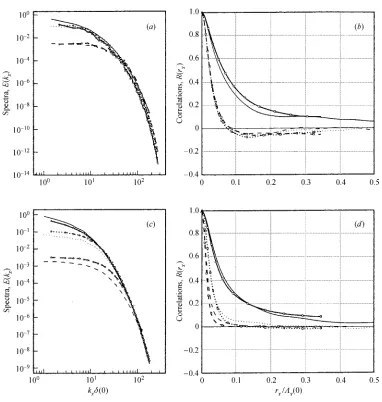
domain sizes are, respectively, 2πandπtimes the channel halfwidthδ. The sufficiency of these numerical parameters has been verified by examining energy spectra and two-point correlations, both before and after the straining (see figure 2). The extra challenge, compared to the conventional unstrained plane channel, of capturing at all times the full range of turbulent scales in a domain whose streamwise extent decreases in time under the APG strain (cf. figure 1b), is revealed in the streamwise velocity correlations at A22t = 0.365 (open-symbol curves) shown in figures 2(b) and 2(d). Although non-zero, values at the maximum-separation rx =Λ(t)/2 are small enough

(approximately 0.1) to imply that all but the very largest streamwise structures have not been significantly affected by the finite streamwise domain. The spanwise integral scales tend to increase somewhat during the straining, but not to the point that the spanwise domain size is inadequate (figures 2f and 2h).

The simulation was performed on Cray T90s at the SDSC/NPACI and DOD/NAVO Centers. A total of 2100 single-processor CPU hours were required to obtain the 21-field average results from A22t = 0 to 0.365, shown below.

3. Results

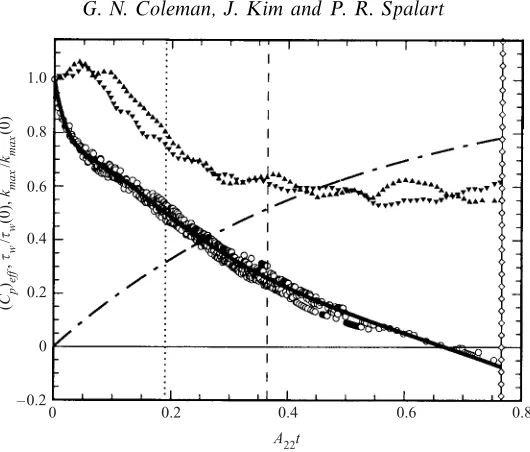
The overall evolution of the flow is illustrated in figures 3 and 4, and catalogued in table 1. In response to the applied strain, coupled with the effective mean pressure variation given by the broken curve in figure 3, the flow is affected at the wall and away from it. The near-wall influence is indicated by the reduction in the skin friction, where the open symbols trace the history of various DNS realizations and the thick-solid curve is an interpolant, given by

τw(s)/τw(0) = exp(c0s) +c1s3+c2exp(c3s) sin(c4s), (3.1) with (c0, c1, c2, c3, c4) = (−3.5433,−0.3127,2.9267,−29.5295,−3.3553) ands =A22t. The wall-stress reversal occurs at A22t ≈ 0.675. We expect this value will be a useful benchmark for testing turbulence models that are to be applied to separating boundary layers. Although the τw = 0 time is not related to a physical separation,

Figure 2(a–d). See facing page for caption.

this time will provide a measure of its ability to faithfully represent attached and separated APG flows of engineering interest. Comparing these tests to those made for the spatial counterpart (e.g. Menter 1992) should give insight into the importance of the features that the flows share (zero skin friction, mean flow reversal) and those only appearing in the spatial case (streamline curvature, mean outflow from the wall dependent on the turbulence instead of imposed, detached/curved shear layers).

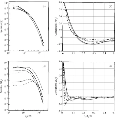
Figure 2. One-dimensional Fourier spectra and two-point correlations: ,ucomponent;

, v; , w. Curves with and without symbols respectively denote A22t= 0.365 results

and unstrained initial conditions at A22t = 0. Streamwise x-direction: (a, b) near centreline,

yw/δ(t) = 0.805; (c, d) near walls,yw/δ(t) = 0.013. Spanwisez-direction: (e, f) near centreline,

yw/δ(t) = 0.805; (g, h) near walls,yw/δ(t) = 0.013. The distance to the nearest wallyw=|y−δ|.

at later times is a symptom of the outer-layer production introduced by the applied strain. This will become clear below, when we discuss the profiles and especially the budgets of the Reynolds stresses.

The evolution of the mean velocity is shown in figure 4 and validates the strained-channel analogy. The curves represent DNS data from the 21-field ensemble for times 06A22t 60.365; the open symbols in figure 4(a–c) are from a single realization at

A22t = 0.77, just after the skin friction has changed sign. (The cost of extending the full average up to A22t = 0.77, by advancing each of the 21 DNS realizations from

0 0.2 0.4 0.6 0.8 1.0

– 0.2

0 0.2 0.4 0.6 0.8

A₂₂t

(

Cp

)eff

,

τw

/

τw

(0),

kmax

/

kmax

(0)

Figure 3.History of effective mean pressure, mean skin friction, and peak turbulence

kinetic energy: , effective pressure coefficient, (Cp)eff = 1−exp(2A11t); 䊊, τw from

21 independent DNS realizations; , equation (3.1) interpolant;䉱and䉲,kmaxfrom (both sides of) a single DNS realization. Vertical lines mark times for which mean profiles are shown in other figures.

A22t δ(t)/δ(0) τw/τw(0) uτ/uc H βeff

0 1 1 0.0495 1.45 0.78 0.19 1.21 0.49 0.042 1.57 2.2 0.365 1.44 0.25 0.036 1.70 5.7 0.77 2.15 −0.05 0.024 2.5 –

Table 1. Global DNS results.

both the reduction of bulk mass flow and wall shear stress (eventually leading to a small mean-flow reversal near the wall) and the increase in the layer thickness found in spatial cases.

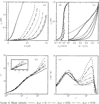
The relatively small amplitude of the applied strain creating these changes is evident in figure 4(b), which depicts the ratio of the strain rate to the mean shear,A22/|∂u/∂y|. This perturbation is such that the effective Clauser parameter βeff increases from −δ∗ucA11/u2τ = 0.78 at A22t = 0, to 5.7 at A22t = 0.365, and then infinity. We are, thus, far from a constant-β, so-called ‘equilibrium’, regime. While the strain becomes increasingly powerful in relative terms as time passes, A22 is at most of the order of 10% of the local shear rate ∂u/∂y (except very near yw = δ, where ∂u/∂y≡0),

even for the A22t= 0.77 conditions, when near the wall ∂u/∂y≈0. The response of the mean flow to the suddenly applied strain is an increase in the shape factor from

H = 1.45 at A22t = 0 to H = 1.70 at A22t = 0.365 and H ≈ 2.5 at A22t = 0.77. The latter value (just afterτw has become negative) is close to theH ≈2.7 found at

0 0.5 1.0

u–/u–_c(0) 0

0.5 1.0 1.5

yw

/

δ

(0)

0 0.5 1.0

yw

/

δ

(

t

)

(a) (b)

0 10–3

(c)

10–1

10–2 ₁₀0 _{– 0.8 – 0.6 – 0.4 – 0.2} (u– – u–_c) /u–_c A₂₂/|∂u–/∂y|

(d) (e)

30

20

10

0

U

+

101 ₁₀2

100 ₁₀1 ₁₀2

y+ _y+

0 10

0 1

100 200 300 400

y+

yw

/

δ

(0)

y

+d

U

+/d

y

+

Figure 4. Mean velocity: , A₂₂t = 0; , A₂₂t = 0.02; , A₂₂t = 0.10; ,

A22t = 0.19; , A22t = 0.28; , A22t= 0.365; 䉫,A22t = 0.77 (single realization). To

aid clarity,A22t = 0.02, 0.10 and 0.28 results are not shown in (b) and (c). Thin-solid curves in

(c) indicate approximation of conserved∂u/∂y. Horizontal line in (e) is 1/κ= 1/0.41. Subplot in (d) shows competing effects of expanding domain and decreasing friction velocity upon wall-normal coordinate in wall units. All velocities measured with respect to reference frame attached to streamwise-moving walls. The distance to the nearest wallyw=|y−δ(t)|.

The mean velocities are shown in an outer scaling in figure 4(c), and com-pared to the variation that would result if ∂u/∂y were to remain constant at a given yw/δ(t) (the thin-solid curves), such that [uc(t)−u(η, t)]/uc(t) = exp(2A22t) [1−u(η,0)/uc(0)]η=η(0), whereη(t) =yw/δ(t) and yw = (δ(t)− |y|) =δ(0) exp(A22t)− |y|. In the present time-developing parallel flow,ηis equivalent to the streamfunction in spatially developing flows, and ∂u/∂y to vorticity. Vorticity is conserved at fixed η

only occur near the wall; as time progresses the influence of viscous and/or nonlinear (i.e. turbulent) effects becomes increasingly important in the outer layer. However, even atA22= 0.77, after the mean flow has changed direction near the wall, the mean velocity of nearly half of the channel is well represented by the conserved-∂u/∂y

approximation. However, conservation of∂u/∂y (vorticity) in the outer layer does not imply that the outer-layer turbulence is only affected by inner-layer changes that have diffused away from the wall; it only implies that the total shear stress remained close to linear. We shall see below that the applied irrotational APG strain immediately alters the structure of the outer-layer turbulence.

In the inner scaling (figure 4d) the mean velocity shows an instantaneous departure from the initial profile, with a rapid increase with time of the wake component (the excess over the logarithmic law, which the initial profile is very close to, for largey+). The initially logarithmic regions of the A22t = 0 and A22t >0 results also differ, as expected for a non-equilibrium layer (unlike for equilibrium APG boundary layers, which are often characterized by inner-layer mean velocities that agree with the zero-pressure-gradient expression in the logarithmic region; see Krogstad & Sk˚are 1995). In contrast to the APG experiment of Nagano et al.(1997), whose wake-component increase was accompanied in the logarithmic region by a uniform shiftbelow the zero-pressure-gradient profile with no change in slope (see also Debisschop & Nieuwstadt 1996), here an initial upward shift is followed by relaxation towards the unstrained initial condition while the slope in the log region increases instantly and monotonically with time (figure 4e). Part of this difference, especially at the earliest times, is an exaggerated response to the impulsive deceleration, compared to the experiments, which enters this type of figure through the friction velocity. Unlike in the spatial case, where the influence of sudden convective changes in the mean flow can propagate upstream through the boundary layer (owing to the interdependence of the free-stream and boundary-layer flows), here the channel turbulence receives no ‘warning’ of the impending discontinuous temporal change. As a result, the initial changes are somewhat more abrupt than those imposed upon turbulence in a spatial boundary layer. In the terminology of Galbraith, Sjolander & Head (1977) (see also Huang & Bradshaw 1995), the perturbation appears to have produced a general rather than progressive departure from the law of the wall. (A progressive departure would have caused y+_dU+_/dy+ _{to gradually ‘peel off’ from the right-hand side of the horizontal}

line in figure 4e.) Unfortunately, we would need much higher Reynolds numbers to rule between general and progressive departures.

Other typical APG characteristics exhibited by the flow are the near-wall reduction, and outer-layer increase, in turbulence intensity, illustrated by the Reynolds shear stress −uv, turbulence kinetic energy k =u_iu_i/2, and vertical velocity variance vv

shown in figures 5(a) and (b). A normalization with the instantaneous skin friction or centreline velocity would magnify the increases and moderate the decreases. The pressure fluctuations (figure 5c) become more intense over the entire channel. Unlike the three-dimensional skewing cases discussed in CKS, the present strain rate is too small to induce an appreciable instantaneous increase in the pressure fluctuations at

A22t = 0 due solely to the impulsive application of the strain (see figures 6c and 17c of CKS).

Another difference between the present and Naganoet al. flows is in the behaviour of the velocity fluctuations in the outer layer: here −uv, k and vv at a given

yw/δ >0.5 all increase, while in the experiment the values at fixedyw/δ exhibit very

0 0.4 1.0 0.5

1.0

yw

/

δ

(

t

)

(a) (b)

(d) (c)

0.2 0.6 0.8 0

0.5 1.0

1 2 3 4 5

0 1

0.5 1.0

yw

/

δ

(

t

)

2 3 0

0.5 1.0

10 20 30 40 50

(p p)1/2_/u2

τ(0) νT/ν

–uv/u2

τ(0) v v/uτ2(0), k/uτ2(0)

Figure 5. Turbulent (a) Reynolds shear stress, (b) kinetic energy and vertical velocity, (c)

pres-sure fluctuations, and (d) eddy viscosity: , A22t = 0; , A22t = 0.19; , A22t =

0.365.

Watmuff (1993) APG the turbulence intensities in the outer layer respond as they do here, increasing at fixed yw/δ as the flow decelerates (see their figures 12c and 12d).

Whether or not the outer-layer turbulence becomes more energetic apparently depends on the history (i.e. magnitudeCp and streamwise variation dCp/dx) of the APG. One

aspect of the relationship between the turbulence and mean fields is illustrated in figure 5(d), which presents profiles of turbulent viscosity νT = −uv

(∂u/∂y). This could provide suggestions for simple turbulence models.

The impact of the strain upon the structure of the Reynolds-stress tensor is reflected in the changes to the ratio of the shear stress to the kinetic energy, a1 =−uv/q2 = −uv/2k, shown in figure 6(a). Although the outer-layer reduction is slight (and in fact non-monotonic), again confirming the robustness of this parameter, the net change is more significant than that induced by the larger pure-skewing strain (i.e. A13 = 0 with A11 = A22 = 0) imposed in CKS (A13 was over twice as large as the present

A22, in terms ofuτ(0)/δ(0)). This is consistent with one of the primary conclusions of

CKS, that turbulent wall layers are more responsive to variations in the streamwise pressure gradient than they are to the introduction of mean three-dimensionality via streamwise variations of the spanwise pressure gradient.

0 0.4 1.0 0.1

(a) (b)

0.2 0.6 0.8 0

0.2

y_w/δ(t) 0.2

0.4 1.0

0.2 0.6 0.8

0 0.4

– 0.2

y_w/δ(t)

–

u

v

/

q

2

Vq

2

/

uτ

(0)

Figure 6. Profiles of (a) stress/energy ratio−uv/q2and (b) turbulent transport velocity

Vq2=vu_iu_i/q2: ,A22t= 0; ,A22t= 0.19; ,A22t= 0.365.

itself,v(uu+vv+ww)/(uu+vv+ww), is plotted in figure 6(b). This quantity measures the velocityVq2 with whichkis transported by the turbulence either toward

(Vq2<0) or away from (Vq2>0) the wall. The tendency for Vq2 to diminish in the

outer layer under the influence of an APG has been observed in the infinite-swept-wing experiment of Bradshaw & Pontikos (1985), and the swept-infinite-swept-wing-strain DNS of CKS. The same tendency holds here: the A11 = −A22 <0 strain leads to significant reduction of the upward transport velocity over the near-wall half of the channel,

yw < 0.5δ. At A22t = 0.77, just after the mean-flow reversal, Vq2 has become even

smaller (and at times negative) than the A22t 6 0.365 values (the A22t = 0.77 result is not shown because of uncertainty associated with forming a third-order statistic from a single instantaneous field). The behaviour ofVq2, when viewed in light of the

corresponding behaviour ofk andνT in figures 5(b) and 5(d), is not inconsistent with

the common assumption that the turbulent flux is proportional to−νT∂k/∂y (Wilcox

1998). However, as we see in figure 7(c), correctly modelling this term appears to be of secondary importance, since changes to the other k-transport processes are even more pronounced.

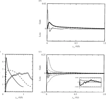
We conclude with Reynolds-stress budgets in figures 7–9. The left-hand plots, (a), show the evolution of the stress component for 06A22t 60.77, while those on the right-hand side, (b) and (c), present the terms responsible for the change. (Incomplete sample is the source of the oscillations atA22t = 0.77 in figures 7a, 8a and 9a.) The curves in the upper-right-hand figures (7b, 8b and 9b) profile the budget terms that are instantly affected by the impulsively applied strain at t = 0; those in the lower right-hand figures (7c, 8c and 9c) show current conditions and the strain-induced changes after a finite time, atA22t = 0.365.

For the general strained-channel flow, the non-dimensionalized transport equations for the Reynolds stresses can be written

∂u_iu_j

∂λ =Pij+Tij+Dij+Πij −εij, (3.2)

1.0

y_w/δ(0)

(a)

(b)

(c) 0

0.5 0.02

0 1

k

/

u

2(0)τ

0

Loss

Gain

1.0

y_w/δ(t) 0

0.5 0.25

0

Loss

Gain

– 0.25

0 1 0

0.004

– 0.004

y_w/δ(0) 1

5

4

3

2

Figure 7. (a) Turbulence kinetic energy k profiles: , A₂₂t = 0; , A₂₂t = 0.365; 䉫,

A22t = 0.77 (single realization). (b),(c) Terms inkbudget at (a)A22t= 0+and (c)A22t= 0.365:

, mean-shear production; , dissipation; , turbulent transport; , viscous diffusion; , velocity pressure-gradient correlation;䊊, applied-strain production (also shown in inset in (c) with expanded vertical scale); thick-solid curve ( ), sum of all terms (≈∂k/∂t) atA22t = 0.365 (also shown in inset). Thin-solid ( ) curves denote terms at

t = 0 (before strain) and are identified by the shaded regions, which indicate change from unstrained initial conditions. Curves in (b) and (c) normalized byU4

ref/ν, whereUref= 1.02uτ(0).

Unstrained initial-field profile subtracted from∂k/∂t in (b) to remove statistically insignificant oscillations. (Note difference in vertical scales of (b) and (c).)

right-hand-side terms are the

production:Pij =−uiv

∂ uj

∂y −u

jv

∂ ui

∂y −u

iuAj −ujuAi,

dissipation: −εij =−

2

Re

∂u_i ∂x

∂uj

∂x

,

turbulent transport:Tij =−

∂ ∂y(vu

viscous diffusion:Dij =

1

Re

∂2

∂y2(uiuj),

velocity pressure-gradient term:Πij =−

u_i∂p

∂xj

+u_j∂p ∂xi

.

The Reynolds numberRe is based on a reference velocityUrefandδ(0);Re is 400 and

Uref is 1.02uτ(0), such that Reτ =uτδ/ν= (uτ(t)/Uref)Re exp(A22t) is initially = 390. The velocity ui and kinematic pressure p fluctuations in (3.2) have been scaled by

Uref, while the spatial variable xi is in units of δ(0). The Reynolds stresses uiuj are

functions solely of time t = λ and the wall-normal coordinate yw. It is convenient

to decompose the production term, in order to distinguish between the direct effects of the irrotational applied strainAij and those arising indirectly through changes to

the rotational mean u(y, t). We separate the total production ratePij into rotational

(i.e. shear) and irrotational (applied-strain) components,Pij =PijS +P A

ij, respectively,

where

PS

ij =−uiv

∂ uj

∂y −u

jv

∂ ui

∂y ,

PijA=−uiuAj −ujuAi. (3.3)

The immediate effect of the impulsively applied strain on the development of the turbulence kinetic energyk is both sudden introduction of the new production term

PA

k = 0.5P

A

ii and a step change in the velocity–pressure-gradient term Πk = 0.5Πii

(recall that in incompressible flow both the mean and fluctuation pressure fields are instantly affected by sudden changes of the mean rate of strain). However, figure 7(b) reveals that the pressure–velocity correlation change (dotted curve) is not nearly as important as the new explicit production (open symbols) provided by the APG strain: the net ∂k/∂t (thick-solid curve in figure 7b) is initially dominated by PA

k; but by

A22t = 0.365, PkA is no longer the sole source of ∂k/∂t. Figure 7(c) shows that the

near-wall kinetic-energy decrease (see expanded-scale inset) is accompanied by large decreases in both mean-shear productionPS

k = 0.5PiiS and dissipationεk= 0.5εii, with

the production falling most rapidly, leading to a negative imbalance. The net positive

∂k/∂t in the other layer, on the other hand, can be traced directly to theA11 =−A22 strain (figure 7c inset).

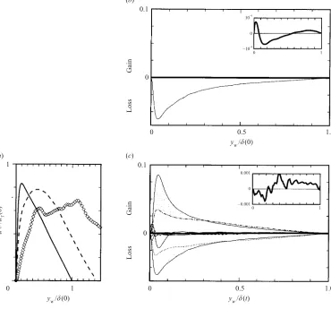
Compared to its initial impact on k, the strain has a much weaker immediate influence upon the −uv shear stress, generating only a slight alteration of −Π12 (figure 8b). The long-term effect is more significant. All the terms in the−uvbudget become smaller near the wall, with the mean shear production −PS

12 (a source of −uv) and velocity–pressure-gradient correlation−Π12 (a sink) experiencing the most obvious changes (figure 8c); a net decrease in −uv occurs since −PS

12 approaches zero faster than−Π12does. The near-balance between−P12S and−Π12is also manifest in the outer layer, where it produces positive −∂uv/∂t. All these changes are an indirect result of the two-dimensional APG strain, since (with A11= −A22) the applied-strain production −PA

1.0

y_w/δ(0)

(a)

(b)

(c) 0

0.5 0.1

0 1

0

Loss

Gain

1.0

y_w/δ(t) 0.5 0

Loss

Gain

0 1 0

10 4

y_w/δ(0) 1

0 0.1

0 1 0

0.001

– 0.001

–

u

v

/

u

2(0)τ

−10– 4 –

Figure 8. (a) Turbulent shear-stress −uv profiles: , A₂₂t = 0; , A₂₂t = 0.365;

䉫, A22t = 0.77 (single realization). (b),(c) Terms in −uv budget at (b) A22t = 0+ and

(c) A22t= 0.365: symbols and normalization as in figure 7. Note that −P12A ≡0 for APG

strain. Unstrained initial-field profile subtracted from−∂uv/∂t in (b) to remove statistically insignificant oscillations.

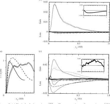
As with ∂k/∂t, the A22t = 0 ‘pulse’ of ∂vv/∂t induced by the APG is primarily due to the new explicit production,PA

22, although the mitigating effect of the velocity– pressure-gradient term Π22 is more important here (figure 9b). The initial ∂vv/∂t is negative over the entire channel. From figure 9(c), we see that at A22t = 0.365 the sign of ∂vv/∂t has become positive over the bulk of the flow, despite the continuing negative contribution of the APG strain, through the explicit production termPA

22 <0. Near the wall, the sum of the velocity–pressure-gradientΠ22, turbulent transport T22 and dissipation −ε22 terms nearly cancel the negative P22A; in the outer layer, the strain has indirectly led to an increase in Π22, which more than offsets the explicit effect of the strain (i.e. PA

22<0). The resulting growth ofvv in turn combines with the nearly constant ∂u/∂y in the outer layer to amplify−uv, via the increased mean-shear production−PS

1.0

y_w/δ(0)

(a)

(b)

(c) 0

0.5 0.01

0 1

0

Loss

Gain

1.0

y_w/δ(t) 0.5 0

Loss

Gain

0 1 0

0.001

y_w/δ(0) 1

0 1 0

0.001

– 0.001 – 0.001 0.02

0.03

– 0.01

0 0.02

– 0.02

v

v

/

u

2(0)τ

Figure 9.(a) Vertical velocity variance vv profiles: , A₂₂t = 0; , A₂₂t = 0.365;

䉫, A22t = 0.77 (single realization). (b),(c) Terms in vv budget at (b) A22t = 0+ and

(c) A22t = 0.365: symbols and normalization as in figure 7. Unstrained initial-field profile

subtracted from∂vv/∂t in (b) to remove statistically insignificant oscillations.

4. Summary and concluding remarks

DNS of time-developing strained-channel flow with a fairly high initialReτ = 390

has been performed as an idealization of a turbulent APG boundary layer. This approach has the advantage of reproducing many of the essential features of the corresponding spatially developing flow (simultaneous skin-friction reduction and distortion due to divergence of outer-layer streamlines) in an uncomplicated parallel-flow geometry. Since statistics vary only in one spatial direction and time, analysis is (and future model testing will be) considerably simplified. A study of how well common one-point turbulence models capture the DNS results is underway (Yorke & Coleman 2004).

streamwise compression ∂U/∂x and wall-normal stretching ∂V /∂y strains directly influence the outer-layer turbulence, causing an increase in turbulence intensity.

The turbulence-modelling challenge for this flow is the manner in which a typical strain field, weak compared to the mean shear, profoundly influences the turbulence in the outer layer –beforealterations diffuse there from the wall region. The DNS results are evidence – albeit tentative, given the spatial-to-temporal idealization involved – that the ∂U/∂x =−∂V /∂y strain introduced by an adverse pressure gradient should perhaps be viewed as a classical ‘extra strain’ (Bradshaw 1988), affecting the turbulence more strongly than an order-of-magnitude estimate (e.g. based on |∂U/∂x|/(∂u/∂y)) would imply. This is demonstrated in the Reynolds-stress budgets by how strain-induced changes to the net ∂τij/∂t are the result of large competing changes to

individual terms. The present results (consistent with those of Spalart & Watmuff 1993) also imply that, while it is apparently valid for some deceleration histories (e.g. Nagano et al.1997), the assumption that the turbulence is unaltered as it convects along outer-layer streamlines until reached by diffusing inner-layer effects should not automatically be made for all APG boundary layers.

This work was sponsored by the Office of Naval Research (grant no. N00014-94-1-0016), Dr L. P. Purtell program officer. Computer resources have been supplied by the SDSC NPACI and DOD MSCR programmes. Professor S. Chernyshenko made useful comments on an early draft of this paper.

R E F E R E N C E S

Alving, A. E. & Fernholz, H. H. 1995 Mean-velocity scaling in and around a mild, turbulent

separation bubble.Phys. Fluids7, 1956–1969.

Bradshaw, P.1973 Effects of streamline curvature on turbulent flow.AGARD-AG-169. Bradshaw, P.1987 Turbulent secondary flows.Annu. Rev. Fluid Mech.19, 53–74.

Bradshaw, P.1988 Effects of extra rates of strain – review.Zoran Zaric Mem. Seminar, Dubrovnik.

Hemisphere.

Bradshaw, P. & Pontikos, N. S.1985 Measurements in the turbulent boundary layer on an ‘infinite’

swept wing.J. Fluid Mech.159, 105–130.

Coleman, G. N., Kim, J. & Spalart, P. R. 2000 A numerical study of strained three-dimensional

wall-bounded turbulence.J. Fluid Mech.416, 75–116 (referred to herein as CKS).

Debisschop, J. R. & Nieuwstadt, F. T. M.1996 Turbulent boundary layer in an adverse pressure

gradient: effectiveness of riblets.AIAA J.34, 932–937.

Galbraith, R. A. McD., Sjolander, S. & Head, M. R.1977 Mixing length in the wall region of

turbulent boundary layers.Aeronaut. Q.28, 97–110.

Hanjali ´c, K. & Launder, B. E. 1980 Sensitizing the dissipation equation to irrotational strains. Trans. ASME J. Fluids Engng 102, 34–40.

Huang, P. G. & Bradshaw, P.1995 Law of the wall for turbulent flows in pressure gradients.AIAA J.33, 624–632.

Krogstad, P.-˚A. & Sk˚are, P. E. 1995 Influence of a strong adverse pressure gradient on the

turbulent structure in a boundary layer.Phys. Fluids7, 2014–2024.

Menter, F. R.1992 Performance of popular turbulence models for attached and separated adverse

pressure gradient flows.AIAA J.30, 2066–2071.

Nagano, Y., Tagawa, M. & Tsuji, T.1992 Effect of adverse pressure gradients on mean flows and

turbulence statistics in a boundary layer. Eighth Symp. on Turbulent Shear Flows, Munich, Germany, September 9–11, 1991.

Nagano, Y., Tsuji, T. & Houra, T.1997 Structure of turbulent boundary layer subjected to adverse

Rogallo, R. S.1981 Numerical experiments in homogeneous turbulence.NASA TM81315. Available

from NASA Scientific & Technical Information ([email protected]).

Rogers, M. M.2002 The evolution of strained turbulent plane wakes.J. Fluid Mech.463, 53–120. Smits, A. J. & Wood, D. H.1985 The response of turbulent boundary layers to sudden perturbations.

Annu. Rev. Fluid Mech.17, 321–358.

Spalart, P. R. & Watmuff, J. H.1993 Experimental and numerical study of a turbulent boundary

layer with pressure gradients.J. Fluid Mech.249, 337–371.

Townsend1961 Equilibrium layers and wall turbulence.J. Fluid Mech.11, 97–120.

Wilcox, D. C.1998Turbulence Modeling for CFD.DCW Industries (www.dcwindustries.com). Yorke, C. P. & Coleman, G. N.2004 Assessment of common turbulence models for an idealized