Abstract— The path planning problem finds a collision free path for an object from its start position to its goal position while avoiding obstacles and self-collisions. Many methods have been proposed to solve this problem but they are not optimization based. Most of the existing methods find feasible paths but the objective of this current research is to find optimal paths in respect of time, distance covered and safety of the robot. This paper introduces a novel optimization-based method that finds the shortest distance in the shortest time. It uses particle swarm optimization (PSO) algorithm as the base optimization algorithm and a customized algorithm which generates the coordinates of the search space. We experimentally show that the distance covered and the generated points are not affected by the sample size of generated points, hence, we can use a small sample size with minimum time and get optimal results, emphasizing the fact that with little time, optimal paths can be generated in any known environment.
Index Terms— Path Planning, Particle Swarm Optimization Algorithm. Robotics, Optimization
I. INTRODUCTION
LANNING a feasible path for a mobile robot is an intractable problem. Yet, it finds applications in robotics, medicine, virtual reality, search and rescue operations and bioinformatics. Motion planning algorithms finds sequence of valid configurations from the free space to form a path, which the mobile robot takes while avoiding collisions. Finding these configurations deterministically becomes a difficult task as the dimensions of the configuration space increases (Reif, [7]).
A lot of solution methods have been proposed to solve this problem. Most of the algorithms find paths that are feasible (Ekenna et al., [3]; Denny et al., [4]; Zhou et al., [10]) while a few try to find the optimal feasible paths (Mac et al., [5], Bayat et al., [1], Wang et al., [9]. Not many have considered how expensive an algorithm is, that is, an algorithm that finds an optimal path as well as seeks to minimize the speed of the planner. This is the motivation of this work.
In this paper, we present an optimization - based algorithm that works with Particle Swarm Optimization
Manuscript received February 27, 2018; revised March 27, 2018. This work was sponsored by Covenant University, Ota, Nigeria.
P. I. Adamu, H. I. Okagbue, P. E. Oguntunde and A. A. Opanuga are with the Department of Mathematics, Covenant University, Ota, Nigeria.
[email protected] [email protected]
[email protected] [email protected]
(PSO) algorithm to find an optimal path. It uses a customized algorithm to generate the coordinates of the search space and passes the result to the PSO algorithm which then uses the coordinate values to determine the optimal path from start to finish.
In our experiment, we considered four environments with different number of obstacles and different population sizes in each environment (Figures 1 – 7). In each of the environment, we considered different number of generated points from the initial point to the final point which is passed on to PSO to find the best ten points that gives the optimal path (Tables 1-3).
In this paper, we considered population sizes 100 (Figures 2, 4 and 6) and 10 (Figures 3, 5 and 7). We used the distance metric to calculate the distances covered in each of the environment and made comparisons (Table 4). Additionally, we compared the coordinates of different population sizes in different environments with obstacles (Figures 8-10). The experiments show that using our algorithm, the population size does not affect the distance covered (Table 4) neither does it affect the coordinates generated from the start point to the end point in any environment (Figures 8-10). Hence, the smallest population size with a minimum time can be used because it gives the desired results. This makes our algorithm to be a fast one in planning a path for a mobile robot. What this implies is that our customized algorithm is able to generate the best points from the initial point to the final position without having to generate so many points and then begin to select from them for the optimal path.
The main contribution of this paper is the introduction of a novel optimization-based method to find a fast algorithm that finds an optimal path for a mobile robot.
II. PRELIMINARIES AND RELATED AREA
A Distance Metrics A distance metric is a function,
(On)ps( , )
s t
R
,
whichcalculates the Euclidean distance between two configurations
s
( ,
s s
1 2,... )
s
n andt
( , ,... )
t t
1 2t
n in the Euclidean space, where ‘On’ is the number of obstacles and ‘ps’, the population size, in the environment under consideration.Mathematically,
2
2
2( )
1 1 2 2
( , )
...
On
ps
s t
t
s
t
s
t
ns
n
A Fast Path Planning Algorithm for a Mobile
Robot
Patience I. Adamu, IAENG, Member, Hilary I. Okagbue, Pelumi E. Oguntunde and Abiodun A. Opanuga
This work uses this metric to calculate the distances covered by the mobile robot from the initial position to the end position in the different environments shown in Figures 1-7. The essence of doing this is to be able to compare the distances covered in the different environments and different population sizes.
B. Path Planning
The path-planning problem is usually defined as follows [11]; “Given a robot and a description of an environment, plan a path between two specific locations. The path must be collision free (feasible) and satisfy certain optimization criteria”. In other words, path planning is generating a collision-free path in an environment with obstacles and optimizing it with respect to some criteria.
C. Global and Local Path- Planning
Global path planning requires the environment to be completely known and the terrain, static. In this approach, the algorithm generates a complete path from the start point to the destination point before the robots starts motion. On the other hand, local path planning means that path planning is done while the robot is moving; in other words, the algorithm is capable of producing a new path in response to environmental changes. Assuming there are no obstacles in the navigation area, the robot moves in a straight line start point and the end point (Figure 1). The robot proceeds along this path until an obstacle is detected. At this point, our path-planning algorithm is utilized to find a feasible path around the obstacle. After avoiding the obstacle, the robot continues to navigate towards the end-point along a straight line until the robot detects another obstacle or the desired destination is reached.
D. Particle Swarm Optimization (PSO)
Particle Swarm Optimization(PSO)is a stochastic global
optimization technique which provides an evolutionary based search. The term PSO refers to a relatively new family of algorithms that may be used to find optimal or near optimal solutions to numerical and qualitative problems. It is implemented easily in most of the programming languages since the core of the program can be written in a single line of code and has proven both very effective and quick when applied to a diverse set of optimization problems. PSO algorithms are especially useful for parameter optimization in continuous and multi-dimensional search spaces. PSO is mainly inspired by social behavior patterns of organisms that live and interact within large groups. In particular, PSO incorporates swarming behaviors observed in flocks of birds, schools of fish, or swarms of bees.
E. Particle Swarm Optimization Algorithm
The procedure is as follows:
Set iteration counter i = 0
Initialize the parameters ω,c1 and c2
Initialize N random particles p1, p2 … pN (also
called positions) and their velocities v1, v2, … vN.
The velocities indicate the amount of change that is applied to a current position (i.e. particle or solution) to arrive at the updated particle (position). The subscripts indicate the particle number in the swarm.
Evaluate the fitness of each particle from the objective function ( n)
i
n F p
f , whereF() is the objective function to be optimized.
Update i n
f
andi n
p
pair as in (1), where i nf
is the pbest andi n
p
the pbest-yielding particle in the i-th generation.
1 1 1
1
[
] if
is better than
[
]
if
is better than
i i i i
i i n n n n
n n i i i i
n n n n
p
f
f
f
p
f
p
f
f
f
(1) That is, compare the current and the previous pbest values and retain whichever is better; also retain the corresponding position (or particle) that yielded the pbest.
Update the global best gbest with best fitness i g
f
. The particle that yields gbest is called the global best particle (or position)i g
p
The pair can be obtained from (2). Update velocities and positions of each particle according to (3) and (4)
1
1 1
(
i i i
n n
v
v
c r
p
in
p
ni)
c r
2 2i(
p
ig
p
ni)
(3)p
ni1
p
ni
v
ni1 (4) For the PSO implemented in this paper, the global best particlep
ig is slightly perturbed to explore positions in its vicinity using (5). This guarantees faster convergence [2] and reduces the chances of the algorithm getting stuck in a local minimum (or local maxima).1 i g
v
p
ig 3i i i
g g
p
v
r
(5) Set i = i + 1 (6) Terminate on convergence (ε is the convergencemeasure) or when the iteration limit is reached. Go to the fourth step.
In (3), r1, r2 and r3 are unit random numbers, c1 and c2 are
constants while ω is an inertia weight which may be adjusted dynamically to control the fineness of the search at different stages of the iteration process [8]. Availability of an expert input in step three increases the convergence speed of the algorithm.
III. FAST PATH PLANNING ALGORITHM
The search space is viewed as a grid which can be described by the Cartesian plane. This search space contains small square-shaped cells whose reference point is at the center. Hence, the coordinate of each cell can be described with the x and y points on the Cartesian plane. In order to avoid ambiguous solutions, we assume that the robot moves along the mid-points of the cells from one cell to another. Another assumption in this process is that the obstacles are placed along the optimal path of the robot motion, that is, the path the robot will take if the search space is free of obstacles (Figure 1). A last assumption is that the start and finish points of the robot motion are fixed. In this case, the starting point is (0.5, 0.5) and the finishing point is (9.5, 9.5) for a 10 x 10 search space or the starting point is (0.5, 0.5) and the finishing point is (99.5, 99.5) for 100 x 100 search space. However, the algorithm is developed in such a way to handle any square shaped search space.
The algorithm we developed using PSO as the base optimization algorithm requires that a valid number, for example 10 for 10 x 10 or 100 for 100 x 100 search space is specified along with a valid integer 1, 2 or 3 for the number of obstacles to be introduced. Thereafter, the algorithm requires that you specify the coordinates of the obstacles corresponding to the number of obstacles specified earlier. Once this is done, the algorithm generates the coordinates of the search space and then uses PSO to determine the optimal path taking into consideration the obstacles introduced earlier. Ordinarily, Particle Swarm Optimization can be used to determine the optimal path between the start and finish point of the robot motion. But, this can only be possible if the coordinates of the search space are known. Practically, it is easier to know the coordinate of the obstacles than the coordinates of the search space with obstacles introduced. Hence, our customized algorithm generates the coordinates of the search space and passes the result to the PSO algorithm which then uses the coordinate values to determine the optimal path from start to finish.
IV. EXPERIMENT
Experimental Set up
The Environment:
We considered four environments: an environment without any obstacle, environments with one obstacle at point (3.5, 3.5), two obstacles at points (3.5, 3.5) and (5.5, 5.5) and three at points (3.5, 3.5), (5.5, 5.5) and (6.5, 6.5) respectively. An environment is a 10 x10 grid terrain. In each of the environment, we ran our algorithm on different population sizes 100, 50, 20 and 10. The algorithm generated the best ten points from the initial point to the end
point in all the populations of the different environments. In this paper, we use the two extreme population sizes 100 and 10 only (Tables 1–3). We then use the tables to draw the graphs for the different environments (Figures 2-6).
A. Enviroment 1: 10 x 10 grid terrain without Obstacles.
The optimal path of running our algorithm in an enviroment without any obstacle is a straight path from the initial position to the final position. The path coincides with the diagonal of the 10 x 10 grid terrain (Figure 1), which is the shortest distance between two nonadjacent vertices of a polygon.
Figure. 1: 10 x 10 grid terrain without obstacle Distance Covered
The distance covered is calculated using the Euclidean distance metric:
2 2
(
start end
,
)
(9.5 5.0)
(9.5 5)
12.73 units
B. Environment 2:10 x 10 grid terrain with one Obstacle at point (3.5, 3.5)
Running our algorithm on this environment with population sizes 100 and 10, We use Table 1 to draw the graphs of Figures 2 and 3.
Table1: Shows the points of sample sizes 100 and 10 Environment with One Obstacle
Population Sizes 100 10
x-cord. y-cord.
x-cord.
Figure 2: Shows the optimal path of population 100
Figure 3: Shows the optimal path of population 10 Distance Covered
i. The distance covered when the population size is 100 (Figure 2):
(2) 2 2
100(start end, ) (2.5009 0.5021) (2.4999 0.4988)
(4.4976 2.5009) (4.5001 2.4991)
2 2
(9.4980 4.4972)
(9.4994 4.5001)
13.87 units.
ii. The distance covered when the population size is 10 (Figure 3):
(2) 2 2
10(start end, ) (2.4972 0.5039) (2.4999 0.4221)
(4.4943 2.4972)
(4.5279 2.4916)
2 2
(9.5014 4.5168)
(9.5125 4.5279)
13.96 units.
C. Environment 3:10 x 10 grid terrain with two Obstacles at points (3.5, 3.5) and (5.5, 5.5)
[image:4.595.80.259.64.189.2]The results of this environment with population 100 and 10 are shown in Table 2 and Figures 4 and 5.
Table 2: Shows the generated points of sample sizes 100 and 10
Environment with Two Obstacles Population Sizes
100 10
x-cord. y-cord.
x-cord.
y-cord. 0.4996 0.5009 0.4912 0.5046 1.5003 1.5034 1.5035 1.4405 2.4999 2.4992 2.4522 2.5455 4.5008 2.5004 4.5624 2.5287 4.5014 4.5003 4.5553 4.4807 6.5005 4.5031 6.4896 4.4993 6.5007 6.4963 6.4897 6.5078 7.4996 7.5034 7.5133 7.4968 8.4995 8.4977 8.3001 8.4999 9.499 9.4993 9.5408 9.5296
Figure 4: Shows the optimal path of population 100
Figure 5: Shows the optimal path of population 10 Distance Covered
i. The distance covered when the population size is 100 (Figure 4):
(3) 2 2
100(start end, ) (2.4999 0.4996) (2.4992 0.5009)
(4.5008 2.4999) (4.5003 2.5004)
(6.5005 4.5014) (6.4963 4.5031)
2 2
(9.4990 6.5007)
(9.4993 6.4963)
15.06 units.
(3) 2 2
10(start end, ) (2.4522 0.4912) (2.5455 0.5046)
(4.5624 2.4522) (4.4807
2.5287)
(6.4896 4.5553)
(6.5078 4.4993)
2 2
(9.5408 6.5007)
(9.5296 6.5078)
15.13 units.
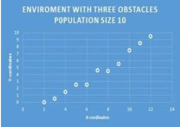
D. Environment 4:10 x 10 grid terrain with three
Obstacles at point (3.5, 3.5), (5.5, 5.5) and (6.5, 6.5)
[image:5.595.57.250.258.601.2]The results of this environment with population 100 and 10 are shown in Table 3 and Figures 6 and 7. Table 3: Shows the generated points of sample sizes 100 and 10
Environment With Three Obstacles Population Sizes 100 10
x-cord. y-cord.
x-cord.
y-cord. 0.4993 0.5008 0.4665 0.4827 1.5002 1.5030 1.5113 1.4915 2.5031 2.4970 2.4399 2.4890 4.5024 2.5024 4.4216 2.5207 4.5003 4.4972 4.4868 4.5528 6.5010 4.5028 6.5026 4.4865 7.5037 5.499 7.5238 5.5060 7.5010 7.5012 7.5094 7.4853 8.4984 8.5004 8.4884 8.5110 9.4990 9.5022 9.4680 9.4668
[image:5.595.298.557.617.725.2]
Figure 6: Shows the optimal path of population 100
Figure 7: Shows the optimal path of population 10
Distance Covered
[image:5.595.56.237.628.756.2]i. The distance covered when the population size is 100 (Figure 6):
2 (4)
100 2
(2.5031 0.4993)
(
,
)
(2.4970 0.5008)
start end
(4.5024 2.5031)
(4.4972 2.5024)
2 2
(6.5010 4.5003)
(7.5037 6.5010)
(5.4990 4.5028)
2 2
(7.5012 5.4990)
(9.4990 7.5010)
(9.5022 7.5012)
=15.07
ii. The distance covered when the population size is 10 (Figure 7):
(4) 2 2
10(start end, ) (2.4399 0.4665) (2.4890 0.4827)
(4.4216 2.4399)
(4.5528 2.5207)
22
(7.5238 6.5026)
(6.5026 4.4868)
(5.5060 4.4865)
2
2
(9.5408 6.5007)
(7.4853 5.5060)
(9.5296 6.5078)
=15.20
Discussion:
A. Comparing the Distances covered in Different Populations:
We compare the distance covered in different population sizes in different environments. Calculating the percentage differences of the distance covered in the different populations as shown in Table 4, we discoverthat with our algorithm, the population sizes does not affect the distance covered.
Table 4: Shows the Population sizes with the distance covered.
Environments One Obstacle Two
Obstacles
Three Obstacles Populatio
n Sizes
100 10 100 10 100 10
Distance Covered
13.8 7
13.9 6
15.0 6
15.1 3
15.0 7
15.2 0 %
Difference
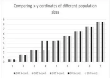
B. Comparing the Coordinates of Different Populations We compare the generated coordinates of populations 100 and 10 in the different environments (Figures 8-10). Series1is 100 x-coordinates, Series 2 is 100 y- coordinates, Series 4 is 10 x- coordinates and Series 5 is 10 y-coordinates. This comparison shows that with our algorithm, the population size does not significantly affect the coordinates generated. Hence, we can make do with the small sample size 10.
[image:6.595.53.237.168.297.2]
Figure 8: Compares the coordinates of the population size 100 & 10 in one-obstacle environment.
Figure 9: Compares the coordinates of the population size100 & 10 in two-obstacle environment.
Figure 10: Compares the coordinates of the
population size100 & 10 in three-obstacle environment
V. CONCLUDING REMARKS
In this paper, we present a new algorithm that seeks to minimize the computation and convergence time of finding an optimal path in a known environment. It uses particle swarm optimization (PSO) algorithm as the base optimization algorithm and a customized algorithm which
generates the coordinates of the search space. Experimentally, we calculate and compare the distances of the optimal paths in population sizes 100 and 10 in each of the three different obstacle environments. We also compare the generated points of the different population sizes. The results show that the population size does not affect the distance covered neither does it affect the coordinates generated from the start point to the end point in any environment. Hence, we can use the smallest population size with small computation and convergence time. This makes our algorithm to be a relatively fast one in planning a path for a mobile robot since we do not need to consider a large population size to get an optimal result. Additionally, the experimental results also illustrate that though PSO algorithms are especially useful for parameter optimization in continuous and multi-dimensional search spaces, with customized algorithm, they are also useful for discrete and 2D search spaces. This can be seen for example in Figure 2, that in trying to avoid the obstacle at point (3.5, 3.5), our algorithm at point (2.5, 2.5) moved to point (3.5, 2.5), then to point (4.5, 2.5) and then finally to point (4.4, 4.5). This is a discrete case. This happened in all the other cases.
ACKNOWLEDGMENT
This research benefited from sponsorship from the Statistics sub-cluster of the Industrial Mathematics Research Group (TIMREG) of Covenant University and Centre for Research, Innovation and Discovery (CUCRID), Covenant University, Ota, Nigeria.
REFERENCES
[1] F. Bayat, S. Najafinia and M. Aliyari, “Mobile robots path planning: Electrostatic potential field approach”; Expert Systems with Applications, vol. 100; pp 68 -78; 2018.
[2] F. Bergh van den, “An Analysis of Particle Swarm Optimizers”. PhD Thesis. Department of Computer Science, University of Pretoria, pp 15 – 30, 2002.
[3] J. Denny, E. Greco, S. Thomas and N.M. Amato, “MARRT: Medial Axis biased rapidly-exploring random trees”. In Robotics and Automation IEEE International Conference on (pp. 90-97), 2014. [4] C. Ekenna, D. Uwacu, S. Thomas and N.M. Amato, Studying learning
techniques in different phases of PRM construction. In Machine Learning in Planning and Control of Robot Motion Workshop (IROS-MLPC), Hamburg, Germany, 2015.
[5] T. T. Mac, C. Copot, D. T. Tran and R. De Keyser “A hierarchical global path planning approach for mobile robots based on multi-objective particle swarm optimization”, Applied Soft Computing, vol. 59, pp. 68-76 2017
[6] U. Paquet and A. P. Engelbrecht, ”Training Support Vector Machines with Particle Swarms”. In Proceedings of International Joint Conference on Neural Networks (IJCNN) Conference, pp 1593 -1598, 2003.
[7] J. H. Reif. “Complexity of the mover’s problem and generalizations”. In Proc. IEEE Symp. Foundations of Computer Science (FOCS), pages 421–427, San Juan, Puerto Rico, October 1979.
[8] G. G. Venu, and K. V. Ganesh, “Evolving Digital Circuits Using Particle Swarm”, In Proceedings oInternational Joint Conference on Neural Networks (IJCNN) Conference, pp 468 – 471. 2003.
[9] B. Wang. S. Li, J. Guo and Q. Chen, “Car-like mobile robot path planning in rough terrain using multi-objective particle swarm optimization algorithm”, Neurocomputing, vol. 282, pp 42-51 2018 [10] Z. Zhou, J. Wang, Z. Zhu, D. Yang and J. Wu, “Tangent navigated
robot path planning strategy using particle swarm optimized artificial potential field”, Optik, vol. 158. pp. 639-651, 2018.
[image:6.595.50.236.345.473.2]