Integral-based Algorithm for Parameter
Identification of the Heat Exchanger
Napasool Wongvanich
∗and Viriya Kongratana
Abstract—This paper develops an integral based method for the system identification and modeling of the heat exchanger. The proposed method formulates the model through the use of integrals, thus rendering a nonconvex optimization problem into simple linear optimization which can be solved through an ordinary least squares method. The convection heat exchanger model is firstly assumed, whereby all the inlet and outlet temperatures are measured or known. Two experiments were conducted. The first involved a series of step responses with incremental heating input, whilst the second involved step responses taken only after the system has cooled down to room temperature. Results show that the proposed method allowed a more complicated model of the heat exchanger to be constructed, whilst still being robust to Gaussian and quantization as well as encoder noises.
Index Terms—Identification, heat exchanger, minimal mod-eling
I. INTRODUCTION
T
HE advent of fast technological advances has furthered the demands for effective energy management in all aspects of life. Thermal energy has emerged the major leader of the modern world, not only in terms of providing useful energy, but to also satisfy the heating and cooling requirements, particularly in industry. Heat exchangers are simply devices that are used to transfer heat between two or more medium of different temperatures, and are used in a variety of industrial applications such as thermal processing plants. Optimal performance of the heat exchangers are dependent on the performances of the controllers themselves, and are usually designed using advanced control algorithms [1]. However, model based controller designs have been favoured in the last few years. This type of controller relies on the incorporation of a simpler mathematical model in the final control law design.The development of a simpler mathematical model for the heat exchanger has also been of interest recently. The main goal in this respect is to synthesize a mathematical model that provides as little complexity as may be possible, whilst concurrently yielding an acceptable precision. The work of Shoureshi [2] showed that a simple fourth order model may have a comparable accuracy to the distributed parameter approach. Fratczak et al. [3] suggest simplification of the heat exchanger model through orthogonal collocation method. Other approaches into model simplification have also been based on the so-called cross-convection model [4]– [6]. Most of these approaches, however, typically assumes a complex model structures first particularly in the parameters
Manuscript received December 07, 2017; revised January 22, 2018 Napasool Wongvanich, and Viriya Kongratana are with the Department of Instrumentation and Control Engineering, Faculty of Engineering, King Mongkut’s Institute of Technology Ladkrabang, Bangkok, Thailand. E-mail: ([email protected], [email protected]).
∗Corresponding author
k1 andk2, then fit this model to the data. And if required, more complex models of spatial temperature distribution is inserted.
This work presents an entirely different philosophy where simplified structures based on the cross convection model is initially assumed. A more sophisticated model of the device is then gradually built through the system identification methodology. This approach also allowed an integral based formulation to be developed that linearizes the optimization and is robust to noise.
II. METHODOLOGY
A. The Heat Exchanger Model
The liquid-liquid heat exchanger is a two chambered device, one for the hot fluid flow with volumetric flow rate of
f1[m3/h], and the other for the cold fluid flow with the flow rate off2[m3/h]. The inlet temperatures are denotedThot,in[◦
C] for the hot fluid, andTcold,in[◦C] for the cooler fluid. The
mathematical symbols for the outlet temperatures areThot,out
for the hot fluid, and Tcold,out for the cold fluid. In general
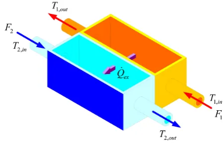
[image:1.595.312.538.441.587.2]the heat exchanger can be described with the schematic of Figure 1 [6]:
Fig. 1. Schematic of the heat exchanger
The basic mathematical description of the heat exchanger model can be derived using conventional first principle considerations. In essence, it is assumed that at steady state each outlet temperaturesThot,outandTcold,outis limited by both
the inlet temperaturesThot,in andTcold,in. This assumption is
due to the principle of heat conservation alone, and does not need placement of further assumptions regarding the spatial distribution of the heat inside the chambers. The following set of differential equations are thus defined:
τ1T˙hot,out(t) +Thot,out(t) =k1Thot,in(t) + (1−k1)Tcold,out(t)
(1a)
τ2T˙cold,out(t) +Tcold,out(t) =k2Tcold,in(t) + (1−k2)Thot,out(t)
where τ1 and τ2 [s] are time constants representing the dynamics of each circuit, andk1andk2are positive constant parameters lumping all the modeling errors including the rheology of the liquid. This model is known to describe well the behaviour of the liquid-liquid heat exchangers. However, for heat exchangers where one of the medium is gas, spatial information regarding the temperature inside the chambers needs to be included, rendering this simple model inadequate for describing the thermal behaviours [6].
B. Integral-based method for system identification of heat exchanger
The differential equation model of Equations (1a) and (1b) are two coupled first order linear equations with constant co-efficients. The signalsThot,inandTcold,inare considered inputs
into the systems, whereas the outlet temperature signals
Thot,out and Tcold,out are considered outputs. To simplify the
system identification problem, it is assumed that both inputs and output signals are known or measured. In practice it is customary to install a thermal sensor at every inlet and outlet chambers in order to completely monitor the heat exchanger. For convenience Equations (1a) and (1b) are rewritten:
˙ y1(t) +
1 τ1
y1(t) =
k1
τ1
u1(t) +
1−k1
τ1
y2(t) (2a)
˙ y2(t) +
1 τ2
y2(t) =
k2
τ2
u2(t) +
1−k2
τ2
y1(t) (2b)
where:
Inputs:u1=Thot,in(t), u2=Tcold,in(t) (3a)
Outputs:y1=Thot,out(t), y2=Tcold,out(t) (3b)
Integrating Equations (2a) and (2b) once with respect to time yields:
y1−y10+a1
Z t
0
y1(t)dt=a2
Z t
0
u1dt+a3
Z t
0
y2dt (4)
y2−y20+b1
Z t
0
y2(t)dt=a2
Z t
0
u2dt+a3
Z t
0
y1dt (5)
where:
a1=
1 τ1
, a2=
k1
τ1
, a3=
1−k1
τ1
(6a)
b1=
1 τ2
, b2=
k2
τ2
, b3=
1−k2
τ2
(6b)
Equations (4) and (5) can be rearranged to yield the integral formulation of ymodel(t):
y1,model=y10−a1
Z t
0
y1(t)dt+a2
Z t
0
u1dt+a3
Z t
0
y2dt (7)
y2,model=y20−b1
Z t
0
y2(t)dt=a2
Z t
0
u2dt+a3
Z t
0
y1dt (8)
where all the integrals appearing in Equations (7) and (8) are computed by the trapezium rule. Substituting y1,model=
y1,data andy2,model =y1,data for allt∈ {t1, . . . , tN} gives a
set of N equations by 8 unknowns which is written in the matrix form:
A p=b (9)
where:
A=
M1|M2
(10)
M1=
1N×1 0N×1 0N×1 1N×1
, M2=
I1,N×3 0N×3 0N×3 I2,N×3
(11)
I1,N×3=
−Rt1 0 y1dt
Rt1 0 u1dt
Rt1 0 y2dt ..
. ... ...
−RtN
0 y1dt
RtN
0 u1dt
RtN
0 y2dt
(12)
I2,N×3=
−Rt1 0 y2dt
Rt1 0 u2dt
Rt1 0 y1dt ..
. ... ...
−RtN
0 y2dt
RtN
0 u2dt
RtN
0 y1dt
(13) p= y10 y20 a1 a2 a3 b1 b2 b3
, b=
y1(t1) .. .
y1(tN)
y2(t1) .. .
y2(tN)
(14)
1M×1=M×1 matrix of ones (15)
0M×N =M×N matrix of zeroes (16)
Solving Equations (9) - (16) by linear least squares yields the parameters a1, a2, a3 and b1, b2, b3. This process deter-mines the identified model for the output temperatures signal
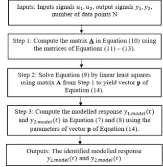
[image:2.595.341.508.491.662.2]y1 and y2 based on the measured data. The algorithm is summarized in a flowchart of Figure 2.
Fig. 2. Algorithm for identifying parametersa1,a2,a3,b1,b2,b3from
the model of Equations (7) - (8)
III. RESULTS ANDDISCUSSION
A. Application to simulated heat exchanger
the heat exchanger model of Equations (2a) and (2b) is used with the following parameters:
k1= 0.93, τ1= 100 (17)
k2= 0.95, τ2= 150 (18)
These parameters are chosen arbitrarily, not based on any physical measurements, and chosen purely to serve the purpose of being proof-of-concept. The simulated responses
y1(t) andy2(t)are sampled at a rate of 200 Hz. Applying the algorithm of Figure 2 yields the following parameters:
a1= 0.01, a2= 0.0093, a3= 0.0007 (19)
b1= 0.0067, b2= 0.0063, b3= 0.0003 (20)
Figure 3(a) compares the identified modely1,model of
Equa-tion (7) to the simulated data. Figure 3(b) compares the identified modely2,modelof Equation (8) to the simulated data
[image:3.595.335.518.91.225.2]of Figure 2. This result shows that the modelled response matches the data very accurately as expected.
Fig. 3. The simulated responsey2.
B. Setup and data acquisition
The setup for the heat exchanger system is shown in Figure 4. The unit used is a liquid-liquid heat exchanger with configurations similar to the one shown in Figure 1. Water is stored in two reservoirs, one for the hot fluid side which is referred to as the hot fluid reservoir in future references; and the other for the cooler fluid side, hereby denoted the cold fluid reservoir. Water from the hot fluid reservoir is pumped into a the heat exchanger system via a 12 V DC motor, and likewise for the fluid from the cold fluid reservoir. A 2 kW heater is connected to the hot fluid chamber to provide the required heating. A variable current source is connected to the heater motor to allow the adjustment of the heat, with 4 mA representing a relative heating level of 0% and 20 mA representing a relative heating level of 100%. These relative percentage representations simplify the computations, and are common in instrumentation engineering. Four resistance temperature detectors (RTDs) are installed at each inlets and outlets of the fluid circuits to measure temperature input and output signalsu1(t),y1(t),u2(t)andy2(t). The overall heat exchanger system is connected to a LabView system via a digital to analogue converter to allow real time access to changing control gains, for data acquisition and viewing the signals. Data from the LabView system is compiled and saved as an.xlsfile, and includes timetand all the input
signalsu1(t),u2(t), y1(t)andy2(t). Matlab is used for all numerical calculations in this work.
Fig. 4. The heat exchanger apparatus
C. Application of the proposed algorithm
Consider an initial data from the heat exchanger unit as shown in Figures 5. The data used is obtained by setting the variable current source to output 8 mA, which is equivalent to the relative heating level of 25%. Note that this data is obtained from an open loop test, representing an initial stage of the modeling. Normally the test being conducted is a step response test, however due to constant heating the accumulation of the heat inside both circuits, the responses ends up increasing in shape of the ramp function. This response in theory still contains many sinusoidal waves, thus provides all the necessary dynamics to do the system identification.
Fig. 5. The responsey2(t)for the case of 25% relative heating.
Applying the algorithm of Figure 2 yields the following parameters:
a1= 0.1009, a2= 0.0327, a3= 0.0671 (21)
b1=−0.0630, b2=−0.0539, b3=−0.0107 (22)
Figure 7 compares the identified modely2,model of Equation
[image:3.595.83.255.295.433.2] [image:3.595.341.508.465.601.2]Fig. 6. The responsey2(t)for the case of 25% relative heating.
D. Extending the model
Note that the linear model of Equations (7) and (8) does not explicitly take into account the constant heating of the 2 kW heater, however some experimental tests can be done to identify such effect. Consider Experiment 1 which is undertaken by changing the heating current by the following functioni(t)defined:
i(t) =
i0, for0≤t≤t1
i1 fort1≤t≤t2
i2, fort2≤t≤t3
i3, fort3≤t≤t4
i4, fort4≤t≤tend
(23)
i0= 8mA, i1= 10mA, i2= 12mA,
i3= 14mA, i4= 16mA (24)
where Tm ∈ {tm−1, tm}, m = 1,2,3 denote the interval
during which the heat exchanger reaches the steady state. This experiment represents a continuous step response tests in which the temperature inside both chambers are allowed to accumulate. For each current level of Equation (24), the algorithm of Figure 2 is applied to identify the parameters
a1, a2, a3 and b1, b2, b3 on the measured data. Figures 7(a) and 7(b) plot the identified a1 and b1. The parameters a2,
a3,b2 andb3 are not shown to conserve space.
The response shown in Figure 7(a) suggests an increasing trend fromi= 8mA toi= 10mA, with a decreasing trend from i = 10 mA to i = 12 mA, then an increasing trend therefter, thereby obscuring an engineer from discerning a pattern or a relationship from this plot. This pattern obscurity could be attributable to the outlier at either i = 10 mA or
i = 12 mA. Nonetheless the pattern can be made clearer through the operation defined:
p1= −1
|p1|
, p=a, b (25)
Notice that Equation (25) is similar to the first expression of Equations (6a) and (6b). The presence of the absolute value operator makes the patterns clearer to discern. Figures 11(a) and (b) show the result of applying Equation (25) to Figures 7(a) and (b). These plots now suggest a power relationship of the form:
fpower(i) =
N
X
j=1
ajij. (26)
Fig. 7. (a) The identifieda1 parameters for the application of i(t)in
Experiment 1 and (b) The identifiedb1parameters.
whereaj are constant to be determined, with respect to the
time constantsτ1andτ2, with an increasing trend of the time constants after i=15 mA as the heating input gets larger. This observation deviates from the actual physics, where the time constant relationship should suggest a decreasing trend as the heating input increases, in line with heat transfer phenomenon. However, a closer look at the data ati=14 mA andi=16 mA reveals that these set of data are in fact obtained with a much shorter timespan than those with smaller heating input, in order to prevent malfunction of the pump motor, which can only physically endures a temperature of up to 60◦C. Such a shorter timespan means that the system may not have yet reached the steady state when its data is used in analysis, resulting in an increasing trend ati=14 mA and
i=16 mA as seen in Figure 8(a) and 8(b).
To ensure that all data sets are of an equal timespan, consider implementing Experiment 2 which is undertaken by changing the heating current byi2(t)defined: defined:
i(t) =
i1, for 0≤t≤t1
0 for t1≤t≤troom temp.
i2 for troom temp.≤t≤t2
0 for t2≤t≤troom temp.
i3, for troom temp.≤t≤t3
0 for t3≤t≤troom temp.
i4, for troom temp.≤t≤tend
(27)
{i1, ..., i4} ≡ Equation (24) (28)
where the time interval{tm, troom temp.}, m= 1,2,3denotes
the time required for cooling down from the steady state of the previous step test to the room temperature, and {troom temp., tn}, n = 2,3 denotes the time required for
[image:4.595.73.252.62.202.2]Fig. 8. (a) The identified time constantsτ1for the application ofi(t)in
Experiment 1 and (b) The identified time constantsτ2 for the application
ofi(t)in Experiment 1.
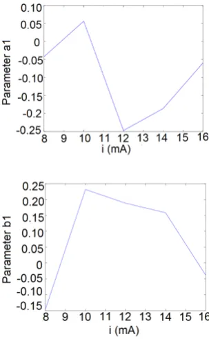
The algorithm of Figure 2 is again used to identify param-etersa1, a2, a3 andb1, b2, b3, as was done for Experiment 1. Figures 9(a) and (b) plot the identifieda1 andb1. Again the parametersa2,a3,b2andb3 are not shown to save space.
Fig. 9. (a) The identified a1 parameters for the application of i(t) in
Experiment 2 and (b) The identifiedb1 parameters.
[image:5.595.93.242.52.297.2]The results of Figures 9(a) and (b) suggest a concave trend for parametera1, and an increasing trend for parameterb1as the current increases. Figure 10(a) and (b) show the result of applying Equation (25) to Figures 9(a) and (b) as was done for Figures 7(a) and (b) in Experiment 1. These plots now
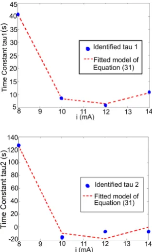
Fig. 10. (a) The identified time constantsτ1for the application ofi(t)in
Experiment 2 and (b) The identified time constantsτ2 for the application
ofi(t)in Experiment 2.
suggest a decaying power relationship of the form:
fpower(i) =
N
X
j=1
αji−j. (29)
The fitting of Equation (29) to Figures 10(a) and (b) now better agrees with the physics, since the time constants τ1 andτ2 now decay with respect to higher inputs, in contrast to results from Experiment 1. Figures 11(a) and (b) plot the relationship between parametersk1 andk2 againsti(t).
Note that these plots share the same trends as Figures 10(a) and (b). This feature is expected, since the parameters
a1andb1as well asa2andb2differ only by a multiplicative constant. Equation (29) is now fitted to Figures 10(a) and (b), as well as 11(a) and (b) using the commandlsqnonlinin Matlab. The matches are shown in Figures 12(a) and (b) for
τ1 andτ2, and Figures 13(a) and (b) for k1 andk2. These results suggest that the proposed method can be used to extend the linear model to include nonlinear effects of a given phenomena. This approach is different from typical approaches in the literature, where the values of the time constants τ as well as k are typically assumed to have certain characteristics and then this ’assumed’ characteristics is fit into the data. The assumed characteristics could also introduce dynamics which are not formally part of the actual phenomenon, and may as well masks any predictable physical laws from being uncovered.
IV. CONCLUSION
Fig. 11. (a) The identified time constantsk1for the application ofi(t)in
Experiment 2 and (b) The identified time constantsk2 for the application
[image:6.595.87.249.56.318.2]ofi(t)in Experiment 2.
Fig. 12. (a) The identified time constantsτ1for the application ofi(t)in
Experiment 2 against the fitted model of Equation (29) and (b) The identified time constantsτ2 for the application ofi(t)in Experiment 2 against the
model function of Equation (29).
convection heat exchanger model is firstly assumed, whereby all the inlet and outlet temperatures are measured or known. The presence of the encoder noise, as well as quantization noise from the ADQ unit, had no effect on the identified parameters nor the resulting model. This result is further testament of the proposed algorithm, suggesting that it could
Fig. 13. (a) The identified parametersk1 for the application ofi(t)in
Experiment 2 against the fitted model of Equation (29) and (b) The identified
k2for the application ofi(t)in Experiment 2 against the model of Equation
(29).
be robust to any type of noise distribution.
Two experiments were conducted to further investigate the effect of the heating current on the identified parameters. The first experiment involved a series of increasing step changes where the heating input current varies linearly. The second experiment is designed whereby the heating current in Experiment 1 is administered only when the system is at the ambient room temperature. The identified time constants were found to have a power relationship where there is a decreasing trend of τ and k as i increases. These results suggest that the proposed method can be used to extend the linear model to include nonlinear effects of a given phenomena.
The investigations undertaken in this paper only take into account the effect of the heating inputs on the time constant
τ and factor k. Investigations into the relationships of the flowf within the chambers, as well as the heating input will be part of the immediate future works.
REFERENCES
[1] R.R. Rhinehart et al., “Editorial – choosing advanced control,” ISA Transactions, vol. 50, pp. 2-10, 2010.
[2] R. Shoureshi, “Simple Models for Dynamics and Control of Heat exchangers,,” in Proceedings of American Control Conference 1983, pp. 1294-1298.
[3] M. Fratczak et al. “Simplified dynamical input-output modeling of plate heat exchangers: a case study”, Journal of Applied Thermal Engineering, vol. 98, 2016.
[4] M. T. Khadiret al.“Modelling and predictive control of milk pasteur-ization in a plate heat exchanger”, Proceedings of the Foodsim, pp. 1294-1298. 2000.
[5] M.A. Abdelghani-Idrissi et al. “Predictive functional control of a counter current heat exchanger using convexity property”,Journal of Chemical Engineering Process, pp. 449-457. 2001.
[image:6.595.91.248.378.637.2]