Complementarity based multiple point collision resolution

Eurographics Irish Chapter

Complementarity Based Multiple Point Collision Resolution

T. Giang,†G. Bradshaw,‡C. O’Sullivan,§

Department of Computer Science, Image Synthesis Group, Trinity College Dublin, Dublin, Ireland

Abstract

Collision detection and response is one of the most extensively researched areas in computer graphics but yet, very little information is available on how to deal with multiple collision situations after they have been detected. In general such topics are quickly brushed over and are small parts of a much larger topic. This paper aims to break this trend and to give a thorough and hopefully informative presentation on how to effectively extract appropriate impulses for multiple point collisions using Linear Complementarity Programming techniques.

1. Introduction

The field of physically based modeling in computer graph-ics research over the last few decades has grown to become quite a substantial subject area. This is partially due to the ever increasing computational speeds of modern day pro-cessors, which has facilitated the growth of feasible real time processing of what once was considered quite com-putationally complex systems. Much research has gone into the reproduction of physically correct behavior of both rigid and non-rigid structures and many dynamics packages have been made available to the general community from such re-search. Cohen et al6_{and Hudson et al}12_{are examples of} pa-pers describing the more popular non-commercial packages available at time of writing (these packages are actually col-lision handling packages, a subset of physically based mod-eling research). Many major computer games and motion picture companies have now started to realise the potential within the area and have started to utilise this vast research in their productions. This in turn has provided a market for many new commercial ventures which have emerged over the last few years to provide such companies with commer-cially viable packages.

One of the most extensively researched topics in physi-cally based modeling has been that of collision detection13 5 15 _{and collision/contact response}2 1 14_{. This paper aims}

† email: [email protected] ‡ email: [email protected] § email: [email protected]

to address in a clear and concise manner the problem of de-termining viable contact impulses during multiple point col-lisions. This is not to be confused with the determination of contact forces which prevent interpenetration. Both ap-proaches are analytically similar and one can be easily ex-tended to incorporate the other. The approach we adopt is analogous to that described by Baraff1_{. However, in this} pa-per we endeavor to provide a more comprehensive treatment of the problem. We first briefly present the basic architecture of how a collision response module fits into the simulation chain and then strive to give an inclusive description from first principles of the underlying solution formulation to the multiple collision point problem.

2. Background

There have been many papers produced in the past years that have in one way or another extensively dealt with the problem of response after a detected collision event14 9 11 17_{. However, many of these papers do not give a thorough} study to the problem of multiple contact collisions or else completely neglect the subject matter altogether. We only concern ourselves with the formulation of multiple collision impulses for rigid body collisions and leave flexible body collision problems for future work.

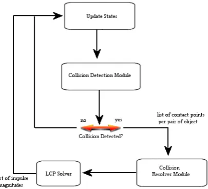
tack-Figure 1: Broad overview of how response module architec-ture fits into a typical dynamics package. The resolver mod-ule is the main modmod-ule which formulates the final problem description which it then passes into the LCP solver.

les this problem by ”inventing” a series of individual non-related impulses that act exclusively on each point of contact which is then incorporated into the matrix of 15 linear equa-tions to be solved for. 11 _{on the other hand suggested the} solution of obtaining an impulse for each point individually and then summing up the resultant impulses that acted on the same body. This however was only suggested for situations whereby a body was in simultaneous contact with multiple other bodies at a single point per contact and the idea was not extended to account for multiple contact points for each pair of contacting bodies.

The most comprehensive treatment to date on the issue of tackling the tricky situation of response impulses for multi-ple point collisions can be found in1_{. The author models} si-multaneous collisions on each colliding body as a collection of impulses acting at each colliding point, each having an effect on how the other behaves. This method is based very much on the same non-penetration techniques presented for resolving contacting forces to prevent inter-penetration in resting contact situations, which is the main body of the pa-per. As such, the bulk of derivative details and assumptions for the simultaneous collision impulse section in the paper are omitted and left to the readers’ own devices. This how-ever, is far from trivial.

3. Task of the collision resolver

Within a typical dynamics simulator, the collision resolver’s job is to determine the outcome of a simulation once a colli-sion has been detected and then to feed back to the simulator

the necessary data to resolve this outcome (see Figure 1). It is the job of the collision detection module in the simulator to detect any potential collisions and to determine the neces-sary contact/collision points along with any other necesneces-sary information needed by the resolver. This information is fed into the resolver which then goes ahead and determines the necessary data that will satisfy the final outcome for the situ-ation at hand. Note that here we ignore all other possibilities like object interpenetration and back-stepping and presume that the collision detection module has taken care of all this for us.

The essential primary data that any collision resolver needs may be as follows:

- the ”common” point of contact - a pointer to colliding object A - a pointer to colliding object B - the normal of contact

- the coefficient of restitution for this collision

The above object pointers point to some rigid body structure whereby all necessary state information about the object can be accessed quickly and conveniently. For non-moveable ob-jects, like walls and floors, the above pointers may point to a dummy rigid body whereby the mass of that body is infinite and the normal of contact is set to point away from the non-moveable structural object(s) (see Figure 2). Also, it may be worth noting that by convention, we consider the normal of contact to always point away from the contacting surface of object B. This is a trivial but important point.

When dealing with simultaneous collisions at multiple points on a body we may consider, for structural conve-nience, this data to be encapsulated within a contact node which itself is part of a list of all colliding points. This is dispatched from the collision detection module to the colli-sion response module.

4. Basic collision impulse assumptions

At collision time tcthere may be two or more bodies

from those points. This will become clearer later on. If there are more than two colliding bodies per point we simply pro-duce a separate contact node for every permutation of pairs of bodies that collide at that point. At the end of this pro-cess we will have a list of contact nodes which correspond to points of contact for each pair of colliding objects. This list, as mentioned previously is then fed into our response re-solver which then solves for the corresponding impulses that act at each collision point. In order to get a better grasp of the final impulse equation formulations, let us initially start from first principles:

Figure 2: contact normal direction of collision between a moveable and non-moveable object at multiple points

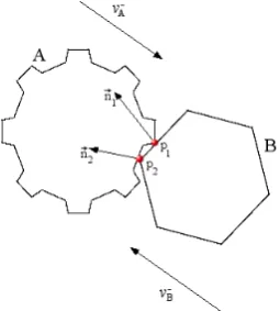
For any pair of bodies, A and B, during a collision at time tc, the ithpoint of contact on body A should be such that it

is equal to the ithpoint of contact on body B (see Figure 3). Let pidenote the ithpoint of contact at time tcon a pair of

bodies A and B so that

pAi(tc) =pBi(tc) =pi(tc) (1)

whereby pAi(tc)and pBi(tc)denote the i

th_{point of contact at}

collision time tcof bodies A and B respectively.

Now let us consider the velocity of each body. At any time t, the velocity of any point on an unrestricted moving body ξmay be expressed as

˙

p_ξ(t) =v_ξ(t) +ω_ξ(t)×(p_ξ(t)−x_ξ(t)) (2)

where v_ξ(t)is the linear velocity of bodyξat time t,ω_ξ(t) is the angular velocity at time t and x_ξ(t) is the center of mass of the object at time t. For notational convenience let us denote(p_ξ(t)−x_ξ(t))as the variable r_ξ(t)from now on. Also, let us represent pre- and post-collision events using

the superscripts− and+ respectively. So the pre-collision velocity of point i at time tcis denoted as ˙p−i (tc)and

post-collision velocity is ˙p+_i (tc).

With this in mind, let us consider what happens during a collision event. According to Newton’s law of restitution for frictionless collisions, at time tc:

v+_rel(tc) =−εv−_rel(tc) (3)

vrelbeing the relative velocity in the normal direction of the

colliding objects which can be expanded to be

vrel=~n·(p˙A−p˙B) (4)

andε being what is known as the coefficient of restitution. This variable, measured between 1 and 0, determines how elastic a resultant collision is and can be viewed as how bouncy the materials from both colliding bodies are. For a perfectly elastic collision,ε= 1, and for a perfectly inelastic collisionε= 0. For a detailed proof please see8.

Figure 3: contacting points and normal directions during collision between two objects. Collision at p1 affects how p2 reacts and vice versa. Both points p1 and p2 are the same for both objects A and B at collision.

to momentum so in fact a more formal definition of an im-pulse would be the instantaneous change in momentum over a very small time period. The direction in whichΨacts re-lates to the direction of the normal of contact. Recall that we said by convention we always consider the normal of con-tact to be pointing away from the surface of object B. All this may be expressed as

Ψ=F∆t=M∆v=f~n (5)

In the above equation, F∆t denotes a large force acting over a very small time period, M is simply the mass of the colliding body,∆v being the change in velocity of the colliding body and f the magnitude of the resultant impulse due to the collision. Though the resultant impulse variable Ψis a vector term, the variable f (the impulse magnitude) is an unknown scalar and is such that f≥0. This is what our resolver wishes to solve for. So, according to Newton’s third law of motion, the final calculated impulse(s) should act positively on one body and equally but oppositely on the other. Let us say that Ψ acts positively on body A and equally but oppositely on body B, thus conforming to Newton’s third law of motion. Thus for body A,ΨA= f~n

and for body B,ΨB=−f~n.

Now, let us deduce the change in velocity due to an ap-plied impulse during a collision at time tc. It is possible to

use the information thus far to derive the change in velocity as an expression in terms of the resultant impulseΨ. Thus the change in velocity,∆v, at any point on a bodyξ due to an imparted impulseΨat time tcis

∆v_ξ(tc) =

Ψξ(tc) M_ξ +I

−1

ξ (tc) rξ(tc)×Ψξ(tc)

×r_ξ(tc) (6)

Where Ψξ(tc)

Mξ is simply the linear component of the change

and the second part, I−1

ξ (tc) rξ(tc)×Ψξ(tc)

×r_ξ(tc)is the

angular component. The variable I−1 is the inverse inertia tensor of the object and all other variables are as described previously. Knowing this, the equation for the post collision velocity of point i on bodyξat time tccan be expressed as

˙ p+

ξi(tc) =p˙

−

ξi(tc) +∆vξi(tc) (7)

We now have v+_rel as a linear function of f .

5. Simultaneous collision points

Recall that during a collision event, v+_rel(tc) =−εv−_rel(tc). We

will need to extend this assumption to fit our multiple colli-sion point criteria. Let us first make the assumption that the

coefficient of restitution,ε, relates to each collision point in-dividually on the colliding body rather than the body as a whole. Since each colliding point on the colliding body in-fluences the other, so too mustε by virtue of relation. So, in short, for each colliding point on the body during a colli-sion event, that point may possess a different elasticity to any other point on that body even though it is part of the same body. Furthermore, the colliding body may be pushed away by a third (or more) body or bodies in a simultaneous, more powerful, collision thus cancelling the effect of the previous collision and breaking the rule in Equation (3). To account for this, let us change the constraint imposed by Equation (3) to one that reflects this situation better:

v+_rel(tc)≥ −εv−rel(tc) (8)

Of course this implies that if v+_rel(tc)exceeds−εv−_rel(tc), then

our impulse magnitude f for that point must be zero as the initial collision contact assumption no longer holds. We can write these constraints down as

v+_rel(tc) +εv−rel(tc)≥0 (9)

f(tc)≥0 (10)

f(tc) v+_rel(tc) +εv−_rel(tc)=0 (11)

From this point onwards, for the sake of clarity, let us drop the tcvariable from our equations as they are going

to get quite messy. Instead, it will be assumed that all equations from here onwards refer to time tc.

Back to the problem at hand. The above three constraints, (9), (10), (11) formulate what is referred to as a Linear Complementarity Problem. More formally, an LCP can be stated as:

Given a known vector b∈Rn_{and a known matrix A∈R}n×n

the problem is to find a vector f∈Rnsuch that

w = Af + b≥0 (12)

f≥0 (13)

fT(w) =0 (14)

or to show that no such vector f exists.

Cottle et al.7_{and Murty}16_{both give excellent detailed} ex-planations of LCPs and various solution methods.†

Our solver’s job is to take constraints (9), (10), (11) and formulate the appropriate A matrix and b vector, giving them to the LCP solver to thus finally solve for vector f , the list of required impulse magnitudes. Let us now extend the post collision velocity equation (7) so that it accounts for simul-taneous multiple colliding points. Recall that we said each impulse acting on each colliding point on a colliding body will influence all other colliding points on that same body. This must be taken into account in the updated equation for-mulation. So updating (7) will gives us

˙ p+

ξi=p˙

−

ξi+

n

∑

j=1

f_ξj~nj

M_ξ +I

−1

ξ

n

∑

j=1

(r_ξj×f_ξj~nj)×rξi (15)

If we substitute equation (15) into equation (4), the resul-tant formulation describes the relative velocity at point i in the normal direction after the collision, taking account of all other influences acting through all other contacting points on the colliding objects.

v+_rel i=v

−

reli+~ni·

n

∑

j=1

fj~nj

MAi

+λAi

n

∑

j=1

(r_A∗_jfj~nj)−

n

∑

j=1

−fj~nj

MBi −λBi

n

∑

j=1

r_B∗_j(−fj~nj)

! (16)

where λAi =r

∗T AiI

−1

Ai , λBi =r

∗T BiI

−1

Bi , fAj = fBj = fj and v−_rel

i is as in Equation (4). Note that we negate the impulse

magnitude f acting on object B in the above formulation so as to conform to Newton’s third law of motion. To neglect to do so would give us an improper model of the resultant impulses acting on each object.

The above equation (16) has been rearranged for nota-tional convenience and clarity. The reader should have no problem in seeing that it was got by simple substitution. Per-haps the only confusing thing is the variables with the∗ su-perscript. Barzel et al3 _{name this ”transformation” as the}

dual of a vector and hence we follow suit here. This formu-lation is just a convenient way for us to express a cross prod-uct of two vectors as a matrix vector multiplication. Equa-tion (17) below might perhaps give a better picture of what is happening. The appendix B in3_{, as well as giving a brief} description of vector dual properties, also gives a very good overview of point behavior on a rigid body which is highly applicable to the equation formulations presented in this pa-per. The reader may want to refer to chapter 4 of Goldstein10 for the proof of why this vector cross product duality relation holds.

a×b=a∗b=  

0 −a3 a2

a3 0 −a1

−a2 a1 0

    b1 b2 b3   (17)

We now take the above equation (16) and substitute for the left hand side of equation (3). This brings us one step closer to obtaining our required b vector and A matrix in our LCP problem. The last thing for us to do is to bring over the right hand side of equation (3) and further rearrange to give:

bi+ n

∑

j=1

fjAi j≥0 (18)

where

bi=v−reli(1+εi) (19)

and

Ai j=~ni·

~n_j

MAi

+λAi(r

∗

Aj~nj)

−−~nj MBi

+λBi r

∗

Bj(−~nj)

!

(20)

Each element i j in the A matrix can be got from the above by straightforward substitution.

The above Equation (20) may still seem a bit overwhelm-ing so let us further simplify the equation by further variable substitution. Let

AAi j= ~nj

M_Ai+λAir

∗

Aj~nj ABi j=

−~nj

M_Bi +λBir

∗

Bj(−~nj)

so that equation (18) can now be expressed as:

bi+ n

∑

j=1

fj~ni· AAi j−ABi j

≥0=wi (21)

6. Conclusions and Future Work

We have set up many experimental animations using the LCP resolution method for simultaneous collisions as de-scribed in this paper and the results to date have been most favorable. Physical plausibility has been maintained, if not improved, for all produced animations. Figure 4 shows stills from an animation of two Stanford bunnies‡falling onto a ramp using the simultaneous multiple collision point reso-lution method as described in this paper. Figure 5 shows the same animation but this time with considered collision points shown. We use a sphere-tree collision detection model 9 4_{so the number of collision points at each narrow phase} collision is vast (as can be seen by yellow points) but how-ever is reduced down to at most an approximate 4 points (these are marked in red). Informal tests have shown that collision response done on multiple collision points simul-taneously rather than on a per point basis in general gives a more pleasing outcome.

Linear Complementarity Programming techniques have been utilised as a solution method in resolving simultaneous contact forces to enforce non-interpenetration constraints1 2_{. However, very little has been seen of them (to our} knowl-edge) when it comes to utilising them as a solution to re-solving simultaneous collision impulses. Baraff’s 1989 pa-per1_{has been the only paper which we are aware of to have} touched on the subject.

For all the technique’s merits however, the necessity of a specialised linear equation solver along with the seemingly complex maths involved may explain why LCP based reso-lution methods for simultaneous collision impulse responses have not been explored or mentioned more in the past. It is our hope that people with little maths background will be able to take what we have presented here and just simply ”plug” each variable in the final formulation into their code or project the necessary data to enable them to account for more than one contact point in a collision. At the very least, we hope that this paper has improved their understanding of how to deal with impulses for multiple collision points.

We are currently in the process of integrating this tech-nique into a dynamics framework and hope in the future to research further into the possibility of speeding up the method by perhaps making the simulation as well as the col-lision detection time critical.

References

1. David Baraff. ”Analytical methods for dynamic sim-ulation of non-penetrating rigid bodies”. ACM SIG-GRAPH, pp 223–232, 1989.

‡ The Stanford bunny model was obtained from Stanford’s 3D scanning repository : http://graphics.stanford.edu/data/3Dscanrep/

2. David Baraff. ”Non-penetrating rigid body simulation.” State of the Art Reports of EUROGRAPHICS’93, Euro-graphics Technical Report Series, 1993.

3. Ronen Barzel and Alan H. Barr. ”A modeling system based on dynamic constraints.” ACM SIGGRAPH, pp 179–188, 1988.

4. Gareth Bradshaw and Carol O’Sullivan. ”Sphere-tree construction using medial-axis approximation.” Pro-ceedings of the ACM SIGGRAPH Symposium on Com-puter Animation SCA 2002. pp 33-40, 2002.

5. Stephen Cameron. ”Enhancing gjk: computing mini-mum and penetration distances between convex poly-hedra.” Int Conf Robotics and Automation, 1997.

6. Jonathan D. Cohen, Ming C. Lin, Dinesh Manocha, and Madhav K. Ponamgi. ”I-COLLIDE: An interactive and exact collision detection system for large-scale environ-ments.” Symposium on Interactive 3D Graphics, pp 189–196, 1995.

7. Richard W. Cottle, Jong-Shi Pang, and Richard E. Stone. The Linear Complementarity Problem. Aca-demic Press, Inc., 1992.

8. Edward A. Desloge. Classical Mechanics, volume 1. Wiley-Interscience, 1982.

9. John Dingliana and Carol O’Sullivan. ”Graceful degra-dation of collision handling in physically based anima-tion.” Computer Graphics Forum (EUROGRAPHICS 2000 Proceedings), pp 239–247, 2000.

10. Herbert Goldstein. Classical Mechanics. Addison-Wesley, Inc., 1971.

11. James K. Hahn. ”Realistic animation of rigid bodies.” In ACM SIGGRAPH, pp 299–308, 1988.

12. Thomas C. Hudson, Ming C. Lin, Jonathan Cohen, Ste-fan Gottschalk, and Dinesh Manocha. ”V-collide: Ac-celerated collision detection for VRML.” VRML 97: Second Symposium on the Virtual Reality Modeling Language, 1997.

13. Ming C Lin. Efficient Collision Detection For Anima-tion and Robotics. PhD thesis, 1994.

14. Brian Mirtich and John F. Canny. ”Impulse-based sim-ulation of rigid bodies.” Symposium on Interactive 3D Graphics, pp 181–188, 1995.

15. Brian Mirtich. ”V-clip: fast and robust polyhedral col-lision detection.” Technical Report TR-97-05, Mit-subishi Electric Research Laboratory, 1997.

16. Katta G. Murty. Linear Complementarity, Linear and Nonlinear Programming. Helderman-Verlag, 1988.

Figure 4: Stanford bunnies falling onto ramps