Online Full Text

(1)



Abstract—For the Wiener degradation failure products, the

effects of life test and degradation test on product reliability evaluation are studied and compared respectively. Firstly, in the cases of no measurement error, measurement error and different number of measurement in the degradation test, the asymptotic variance of the estimated p-percentile of the product’s lifetime distribution is given, and we research the influence of measurement error on evaluation accuracy. Furthermore, under the constraint that the total experimental cost does not exceed a predetermined budget, we set the asymptotic variance of the estimated p-percentile of the product’s lifetime distribution as reliability evaluation accuracy index. In the same evaluation accuracy, we compare the optimal design problem in time censored life test with that in degradation test in different situations. Researches have shown that compared with the life test, the degradation test has obvious advantages for improving the accuracy of product reliability evaluation, which can significantly reduce the sample size and fully use the advantages of test time. The research in this paper can provide reference value for the optimization of long-life product reliability evaluation.

Index Terms—Wiener process; life test; degradation test;

Fisher information; optimal design.

I. INTRODUCTION

n order to clarify the life distribution of the product, estimate the reliability indicators of the product, study the failure mechanism of the product, we often conduct reliability tests. Traditional reliability test evaluations use life tests to estimate parameter distributions from life data. However, with the continuous extension of product life, the general life test cannot obtain enough life information under the limited time and constraints of cost. Then people propose a degradation-based reliability technology. Degradation-based reliability technology provides a new technical approach to

Manuscript received March 7, 2019; revised March 27, 2019. This work was supported in part by the National Natural Science Foundation of China under Grant Nos. 71371183 and 71071158.

Xinyu Ma, 1995.3, female, master, College of Systems Engineering, National University of Defense Technology, Changsha, 410073, major research direction reliability engineering, phone: 18890067587; E-mail: [email protected].

Guang Jin, 1973.1, male, researcher, Ph.D., College of Systems Engineering, National University of Defense Technology, Changsha, 410073, main research direction: reliability engineering, prediction and health management, system testing and evaluation, E-mail: [email protected]

solve the problem of long-life product reliability assessment. Through the degradation test, from studying the product failure mechanism, we analyze the product failure correlation and degradation failure law to obtain performance information. There are some studies on life test and degradation test. A detailed discussion of the maximum likelihood estimation of the failure time data is given by Lawless[1]. Lu and Meeker[2] discuss the method of using degraded data to estimate the failure time distribution. Lu and Meeker[3] define the relative efficiencies to compare the asymptotic efficiency of degradation analysis with that of traditional failure time in life analysis.

We generally consider that, compared with the life test, the test data can be fully utilized by degradation test and the degradation process modeling, and high reliability evaluation accuracy can be obtained. However, the current conclusions are mainly qualitative judgments and lack of quantitative comparative studies. In this paper, the asymptotic variance of product’s reliable life (the percentile of the product’s lifetime) is used as the accuracy index. The quantitative comparison study is carried out, based on the role of life test and degradation test in the modeling and evaluation of long-life product reliability. Firstly, in the cases of no measurement error, measurement error and different number of measurement in the degradation test, we give limit form of asymptotic variance of reliable life of products based on degradation test data. Then we study the optimal design problems for degradation tests and life tests. The optimal variables are sample size and censored time. With constraint of total experimental cost, the optimal settings of these variables are obtained by minimizing reliable life assessment accuracy. Finally, we compare the result in time censored life test with that in degradation test under different number of measurement.

II. WIENER DEGRADATION PRODUCT RELIABILITY MODEL

We know that the lifetime of classical Wiener degradation failure product obeys inverse Gaussian (IG) [4], and its distribution function and density function are respectively

2 2

( ) t l exp l t l

F t

t t

  



 

 

     

 _ _ _ _ _ _

 

    (2.1)

2 2 2 3

( )

( ) exp

2 2

l l t

f t

t t

  

  

 _ _

  (2.2)

Comparison of the Effectiveness of Degradation

Test and Life Test Based on Wiener Degradation

Failure Product

Xinyu Ma,GuangJin

(2)

p

 is 100 th

p percentile of the product’s lifetime distribution,

and ˆ 1

( ) p F p

 _  _{. By using the}_ _{-method, the asymptotic}

variance of 100 th

p percentile of the product’s lifetime distribution _Aver(ˆ_p₎ is

1 2 1 ˆ Aver( ) ( ( ( ))) p

f F p

  _ H I H   (2.3) Where

1 2 q

F F F

   _ _ _   _ _      H

which is the value of the first-order partial derivative of inverse Gaussian distribution function;

1 1

2 2 2 2 2 2

2 2

1 1 2 1 1 1 2 1

2 2 2 2

2 2

2 2 2 2

2 2 2 2 ( ) ( ) ( ) ( ) ( ) E = ( ) q q q q q q

L L L L L L

E E E

L L L L

E E L L E                     _ _  _    _ _ _    _ _ _   _ _ _       _ _   _ _                            _   _   _   _          I

which is Fisher information matrix.

III. RELIABILITY MODELING BASED ON LIFE TEST DATA

Considering the case of the timing censored life test, supposing the sample size is n, the censored time is T, and the failure time data is X₁X₂ X_DT , D is the number of failed sample. Denoted X as the sample data, the likelihood function is [5]

2

2 2

1/ 2 ₂

2 3 2

1 1 1 ( , ) ( ) ( ) ( ) exp 2 2 n D l D i

i i i

L l T e T l

T T x l l x x                     _  _  _  _                      



x

Calculate the second order partial derivative of the log-likelihood function for the parameter  and 2_{, we get}

2 2

2 2 2

2 2

2 2 2 2 2 3

1

2 2

1 11 1 1 1 2 2 2 2 11

2

2 2 2

2

2 1 2 2 2 1

2 2 2 3

( )

( ) 2( ) ( )

2

( ) ( ) ( ) ( ) ( ) 4

( )

1 ( , , )

4 4

( ) ( )+ ( )

( ) ( )

1 ( ,

D i

i i

l l

T T T T T T T T

l l l

T T T T T T

x l L Dl

n D x

l

L L e e M

F T

l l

e M e e M

F T                            _{ }  _ _{  }      _ _ _ _ _         _       



2 2 2 2 2 2

1 1 2 2 2 2 1

2 2

, )

2

( ( ) + ( ) ( ) )

( )

(1 ( , , ))

l l

T T T T T

l

L e e M

F T                          2

2 2 2

2 2

2

2 2

2 1 22 1 1 2 2 2

2 2 2

1

2 2 2

2

2 2 2 2 2 2 2 22

2

2 2

2

1 2 2 2 2 2

2

( ) ( ) ( ) ( )

+( )

1 ( , , )

4

( ) ( ) ( )

1 ( , , )

2

( ( ) ( ) ( ) )

(1

l

D T T T T T T

i i

l l l

T T T T T T T

l l

T T T T T

l

L L e

x L

n D

F T

l

e M e M e M

F T

l

L e e M

                                              _{ } _ _ _           



2 2 ( , , ))

F T  

      2 2 2 2 2 2 2

2 2 1 2

2 2 2 2 2 2

1

2 2

1 12 2 12 1 1 2 1 2 2 2 2

2 2

2

2 2 2

2 3 2 2 2

( )

( ) ( )

( ) ( ) 1 ( , , )

2

( ) ( ) ( ) + ( )

( )

1 ( , , )

4 2 2

( ) ( )

l D

i T T T T

i

l l

T T T T T T T T T

l l

T T T

x e M M

L l

n D

F T

l

L e M L L e

F T

l l l

e e M

                                _  _{ }       _ _ _{ }  _             



2 2 2 2 2 2 2 1 2 2 2

1 2 2 2 2 2

2 2

1 1 2 2 2 2 1

2 2

( )

1 ( , , )

2

( ( ) ( ) ( ) )

(1 ( , , ))

2

( ( ) + ( ) ( ) )

( )

(1 ( , , ))

l

T T

l l

T T T T T

l l

T T T T T

e M

F T

l

L e e M

F T

l

L e e M

F T                                               

Where



 

 is the density function of the standard normal distribution,

 

( )

is the standard normal distribution function, in addition,

1 2 2 2

1 1

1 2 2 3 2 2

2 2

1 2 _{2 3} 2 2 2

2 2

1 1

11 2 2 _{2 5} 12 2 2 3

2 1 22 1 1 ( ) ( ), ( ) ( ), 1 ( ),

2 ( )

1

( ), = ,

2 ( )

3

( ), ,

( ) ₄ ₍ ₎ 4( )

T T

T T T

T T

T

y y y l T l T

T T

T

L l T L

T

M l T M L

T

L l T L

T L          _   _    _   _    _   _                                              , , 2 2 11

2 2 2 2 5

2 2

12 2 2 3 22 2 22

3

0, ( ),

( ) 4 ( )

, .

4( )

T T

T

T T

T T T

M l T

T T

M M L

 _   _                       

Then, in the time censored life test, the variance-covariance matrix of the model parameters’ maximum likelihood estimation is 1 2 2 2 2 2 2 2

2 2 2

( , ) ( ) L L E L L           _ _    _ _{ }     _ _           

I (3.1)

2 2

2 ˆ, ˆ

( F, F)    

  _ _

 



 

H (3.2)

Where

2 2

2 _{2 3} 2 _{2 3}

2 2

2 2 2 2

1 1 1

(1 ) ( ( 1)) (1 )

2 ( ) 2 ( )

1 2 1

( (1 )) ( (1 ))

( )

p p p

p p p p p p p F e e                          _ _ _ _ _ _        2 2 2

2 2 2 2

2

2 2

1 2 1

( ( 1)) ( (1 ))

1

( (1 ))

p p p p p p p p F e e                       _ _ _ _{ } _ _   

Substituting the H and I matrices into the formula (2.3), the asymptotic variance of ˆ

p

(3)

IV. RELIABILITY MODELING BASED ON DEGRADATION TEST

DATA

Suppose the sample size is n, the test duration is T, the number of measurement for sample

i

is

m

_i, the observation interval is

ij t

 and the observed data is x_ij, which is the performance change of sample i between two adjacent measuring times.

A. Case 1: without measurement error

When there is no measurement error, the likelihood function of the degradation test data is as the following, according to the independent increment property of Wiener process: 2 2 2 2 1 1 ( ) 1

( , ) exp[ ]

2 2 i m n ij ij

i j _ij ij

x t L t t               



After calculating log likelihood function, the second order partial derivative of the log-likelihood function for the parameter



and



2_are

2 2 2 l nT    _{ }  2 2

2 2 2 2 2 3

1 1

( )

( ) 2( ) ( )

i

m n

ij ij

i j ij

x t l mn t





 



    _ _ 



 2

2 2 2

1 1 ( )

i m n ij ij i j x t l



 

 



    _  



Expected values are 2

2 2

( l) nT

E

 

 _{ }



2

2 2 2 2

( )

( ) 2( )

l mn E



 _{ }  2 2

( l ) 0

E  

 _

  So the Fisher information is

1 2 2 2 2 0 ( , ) 0 2( ) nT mn                   I

The estimation accuracy of ˆ p  is

 

2

2 2 4

2 3 2 2

2 2

1 ˆ

Aver( )

(1 ) 2

2 exp[ ] [ ( ) ( ) ]

p p p p p f F F nT mn                            

H I H

B. Case 2: with measurement error

For the convenience of description, only consider equal measurement interval. That is to say, for each sample i and measurement time j , observation interval  t_ij  . The

number of measurements is the same for each sample, which is

m

and the observation interval = /T m . Let the measurement error (standard error) is _R. For each sample i, the degradation test data is written as   Xi



xi_,1, ,xi m_,



T, then the likelihood function of parameters



, 2_, 2

R  is [6]

2 2 2 2 ₂

1 2

1

( , , ) (2 )

1

exp ( ) ( )

2 mn n R R n T i i i R

L   

      _           _ _{   } _{    }         



X 1 X 1

There,

1

is m-dimensional column vector with all elements being 1. 2 2 R D P     

1 0 0

0 1 0

0 0 1 m m

T D m               

, 2 1 0

1 2

1

0 1 2 _{m m}

P     _        _   

Set the measurement accuracy index 2 2 R







 , we get 1

D P    

The second order partial derivative of the log-likelihood function for the



,



2 and 2

R  are 2

1

2 2( ) ( )

T R

L n _ _

 





    

 1 1

2

1 1

2 2 4

1 1 1 6

1

1 =

( ) 2

1 ( ) ( ) R n T i i i R L n

tr D D D D                          _ _           



X 1 X 1

2 4 2

1 1 1

2 2 4 8 6

1 6 1 2 1 1 8 1 4

1 1 1 10

1

2 =

( ) 2 2

1

( ) ( )

2

( ) ( )

R R R R

n T i i i R n T i i i R n T i i i R

L mn n

tr D D D

D D D             _{ } _{ }   _{ } _{ }                 _ _ _{     } _{ } _    _ _                                



X 1 X 1

2 1 1 2 4 1 1 1 4 1 1 ( ) ( ) 2 1 ( ) ( ) 2 n T i i R n T i i R L D D                  _{ } _ _ _{ } _{   }         



1 X 1

X 1 1

2 1 2 4 1 1 4 1 2 1 1 6 1 2 1 1 6 1 1 ( ) ( ) 2 1 ( ) ( ) 2 ( ) ( )+ 2 ( ) ( ) 2 n T i i R R n T i i R n T i i R n T i i R L D D            _ _{ }   _{ } _             _{ } _ _{     }                       



1 X 1

X 1 1

1 X 1

X 1 1

2 2

1 1 1

2 2 6 4

1 1 6

1 2

1 1 1 8 1 1 2 1 ( ) ( ) ( ) ( )

R R R

n T i i i R n T i i i R L n

tr D D D D D D            _{ } _{ }               _{ } _ _ _ _ _     _ _                      



X 1 X 1

We can get the H matrix as

2 2 2 2

2 2

ˆ, ˆ, ˆ

( , , )

R R R

F F F

         _ _ _        H Where 2 2 2

2 2 2 2

2

2 2

1 2 1

( ( 1)) ( (1 ))

1

( (1 ))

(4)

2

2 2 3 2

2 2 2 3

2

2 2 2

1 1

(1 ) ( ( 1))

2 ( )

1 1

(1 ) ( (1 ))

2 ( )

2 1

( (1 ))

( ) p p p p p p p p p p F e e                     _     _ _ _ _         2 0 R F   _ 

By substituting the H and I matrices into the formula (2.3), the asymptotic variance of the ˆ

p

 under the degradation test can be calculated. When the numbers of measurement are 1, 2 and 3 respectively, limit form of measurement accuracy of degradation test and the asymptotic variance of the ˆ

p  is shown in the following.

When the number of measurement is 1

For each sample is only measured once, that is m=1, there is

1 2

2 2

2 2 2 2 2 2

2

2 2 2 2 2 2

1

0 0

1 2

1 1

( , , ) 0

2( ) (1 2 ) ( ) (1 2 )

1 2

0

( ) (1 2 ) ( ) (1 2 )

R

nT T

n n T

T T

n T n T

T T                   _                          I

When measurement accuracy 0, the Fisher information matrix can be written as

1

2

2 2

2 2 2 2

2 2 2 2 2

0 0

( , , ) 0

2( ) ( )

2 0

( ) ( )

R

nT

n n T n T n T

                              I

We can find that the equation is a singular matrix. This means when the number of measurements is 1 and every sample is measured at the same time, we cannot use the test data to distinguish between the diffusion parameters and the measurement error. Therefore, in the case of measurement errors, different measurement times are required for different samples.

When the number of measurement is 2

Each sample is measured twice, i.e. m2, and we can get

2 2 2 1 ( ) 1 L nT E           2 2

( L ) 0

E        2 2

( ) 0

R L E       

2 2 3 4

2 2 2 2 3 3

1 16 96( ) 256( ) 240( )

( )

( ) ( ) (1 ) (1 3 )

L n T T T T

E    

     

    

 

  

2 2 3 4

2 2 2 2 3 3

4 56 288( ) 672( ) 576( )

( )

( ) (1 ) (1 3 )

R

L n T T T T T

E    

      

    

  

   

2 2 2 3 4

2 2 2 2 3 3

20 256 1152( ) 2304( ) 1728( )

( )

( R) ( ) (1 ) (1 3 )

L n T T T T T

E =    

     

    

 

  

We can get 2

2 2 2 2 0

lim ( )=

( ) ( ) L n E       2

2 2 2 2 0

4

lim ( )

( )

R

L n T

E          , 2 2

2 2 2 2

0

20

lim ( )=

( R) ( )

L n T

E

  

 



We can obtain that when the measurement accuracy 0 (that is, the measurement error is particularly small relative to the diffusion coefficient), the Fisher information matrix is

1 2 2

2 2 2 2 2 2

2 2 2 2

2 2 2 2 2 2

2 2 2 2

0 0

4 5( ) ( )

( , , ) 0 0

( ) ( )

4 20 ₀

0 4 ( ) ( ) R nT nT

n n T T

n n

T T

n T n T

n n                 _ _           _ _            _ _            I

The limit of estimation accuracy is

 

2

2 2 4

2 3 2 2

2 2

ˆ Aver( )

(1 ) 5

2 exp[ ] [ ( ) ( ) ]

p p p p p f F F nT n                _ _           

H I H

From the Fisher information matrix under the measurement accuracy 0, when there is no measurement error, if the reliability model parameters are estimated in a way with measurement errors, the accuracy of the estimation will be lower than the actual result without measurement errors. When the number of measurement is 3

Each sample is measured three times, that is m3, and the expectation value is

2 2

2 2 2

1 16 60( )

( )

(1 2 )(1 4 2( ) )

L nT T T

E  

                 2 2

( L ) 0

E        2 2

( ) 0

R L E       

2 2 3

2 2 2 2 3 2 3

4 5 6

3 2 3

7

3 2 3

3 126 2214( ) 21060( )

( )=

( ) 2( ) (1 2 ) (1 4 2( ) )

116964( ) 379080( ) 659016( )

(1 2 ) (1 4 2( ) )

454896( )

(1 2 ) (1 4 2( ) )

L n T T T

E

T T T

T                                  _   _               _

2 2 3

2 2 2 2 3 2 3

4 5 6

3 2 3

7

3 2 3

9 342 5346( ) 44388( )

( )=

( ) (1 2 ) (1 4 2( ) )

210924( ) 577368( ) 857304( )

(1 2 ) (1 4 2( ) )

524880( )

(1 2 ) (1 4 2( ) )

R

L n T T T T

E

T T T

T                                   _    _      _         _

2 2 2 3

2 2 2 2 3 2 3

4 5 6

3 2 3

7

3 2 3

72 2592 37908( ) 289656( )

( )

( ) ( ) (1 2 ) (1 4 2( ) )

1236384( ) 2939328( ) 3674160( )

(1 2 ) (1 4 2( ) )

1889568( )

(1 2 ) (1 4 2( ) )

R

L n T T T T

E

T T T

T                                 _   _ _ _              _ There 2

2 2 2 2 0

3

lim ( )=

( ) 2( )

L n E       2

2 2 2 2 0

9

lim ( )

( ) R

L n T E          2 2

2 2 2 2

0

72

lim ( )=

( _R) ( )

L n T

E

  

 



(5)

1 2 2

2 2 2 2

2 2

0 2 2 2 2

2 2 2 2 2

2

2 2 2 2

0 0

3 9 8( ) ( )

( , , ) 0 = 0

2( ) ( ) 3 3

( ) ( )

9 72 ₀

0

3 18

( ) ( )

R

nT

n n T T

I

n n

T T

n T n T

n n

 

  

 



   

   

  _ _

   

    

   

  _ _



   

 

 

 

 

2

2 2 4

2 3 2 2

2 2

ˆ Aver( )

(1 ) 8

2 exp[ ] [ ( ) ( ) ]

3

p p

p

f

F F

nT n

 

  

 

   



  

_ _  

  

   

 

H I H

V. CASE STUDY

In order to compare the effectiveness of degradation and life test, the life test data and the parameter estimation based on the degradation test data are represented by subscripts T

and D, respectively. As can be seen from the fourth section, when the number of measurements is 1, the Fisher information amount is a singular matrix, so the following is only studied when the number of measurements is 2 or 3. We study the effect of measurement error on reliability assessment and compare the effects of time censored life tests with degradation tests on reliability assessment. Without loss of generality, in the following study, we set the drift parameter

=1

 , diffusion parameter =1 , and product failure threshold 1

l for the Wiener degradation model. A. Effect of measurement error 2

R

 on degradation process modeling

When test duration =1T , the number of sample size nD=1,

figure 1 and 2 show the relationship between measurement error and the drift parameter as well as diffusion parameter estimation accuracy of in degradation test. rom the figure, we find that when the measurement error increases, the estimation accuracy of the drift parameter increases linearly, which is proportional to the measurement error, while the estimation accuracy of the diffusion parameter increases nonlinearly and the acceleration speed increases, which in proportion to the second of the measurement error. Fixed measurement error, the higher the number of measurements, the higher the accuracy of parameter estimation. Ideally, cut back the measurement error and raise the number of measurements can obtain higher accuracy.

[image:5.595.48.289.51.200.2]

However, under practical engineering practice, due to cost and instrument limitations, measurement errors cannot be reduced indefinitely or the number of measurements cannot be increased indefinitely. Further we discuss the effect of measurement error on the asymptotic variance. The figure 3 shows the measurement error and the asymptotic variance (reliable life) estimation accuracy curve, we take that the number of measurements is 2 and 3, and p is 0.5 and 0.9 respectively. We can see from the curve in the figure that when the number of measurements is constant, the smaller the p value, the higher the precision; when the parameter p is constant, the more the number of measurements, the higher the accuracy is.

[image:5.595.315.528.58.439.2]

Fig. 1 Effect of measurement error on var( )



ˆ [image:5.595.313.530.265.623.2]

Fig. 2 Effect of measurement error on var(



ˆ2)

Fig. 3 Effect of measurement error on

Aver(



ˆ

_p

)

B. Degradation test plan optimization

(6)

Suppose the price of a single sample is 0

c , the labor and public resource cost per unit time is

p

c , the cost of each measurement is

m

c . If there are

n

samples to be tested, each sample is measured m times, and the test duration is

T

, then the total cost of degradation test is

0

( ,

, )

_p _m

TC n



t m



c n c m t



 

c mn

Generally, in degradation test, the cost of each measurement c_m is not fixed, but is related to the measurement error _R of the test. Usually, the smaller the measurement error is, the higher the measurement accuracy is, and the higher the cost per measurement. Here we assume that

m

c and R

 are inversely proportional, that is c_mw



_R. In reference [7], assuming the price of a single sample c₀80, the human and public resource costs per unit time

0.07 p

c  ,w1, so the total cost in the degradation test is

1

( D, D, ) 80 D 0.07 D D

R

TC n m T n T m n



  

[image:6.595.68.283.344.520.2]

From this, when there is one sample in the degradation test at a fixed censoring time T 1, the relationship between the measurement error and the measurement cost is as follows:

Fig. 4 Relationship between



_R and total cost In the reliability test, under the given cost constraint, the higher the accuracy of the reliability index is, the better the model is. The asymptotic variance of the product can be used as the optimization target, and the test cost is used as the constraint. Consider taking degradation test on the same batch of products and taking the parameters p0.9, censored time

1

T and the number of measurements m3. The total test cost is required to not exceed 4000, and we use genetic algorithm [9][10] to get the degradation test optimal scheme:

measurement error 2 _0.0388 R

  ,

sample size n_D 42,

At this time, asymptotic variance reaches the minimum and

Aver(



_p)=0.1710

We can see that in short censored time, if we need to achieve better evaluation accuracy, you need higher measurement accuracy.

If there is no restriction on the test time, when censoring time is T1089, the sample size is nD48 and measurement

error is 2

2.9563 R

  , the asymptotic variance of ˆ p

 reaches minimum and Aver( )=0.075p . We can see that even if the measurement error is large, the influence can be compensated by a long test time, and a high evaluation accuracy is obtained. C. Comparison on degradation test and time censored life test

A large number of theoretical studies and practices have shown that degradation testing can make full use of experimental information and improve reliability modeling and evaluation accuracy compared with life test. In order to quantitatively compare the pros and cons of degradation test and life test in reliability modeling and evaluation, based on reference [7], we set the cost of each measurement for the life test c_m 10, so the total cost in the life test is

( , )_L 90 _L 0.07

TC n T  n  T

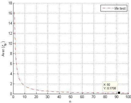
When the censored time is 1, we find that to achieve the same asymptotic variance as degradation test, figure 4 shows the relationship between the asymptotic variance and the sample size. The life test sample amount required is ₉₂

L

n  , when its accuracy reach the same asymptotic variance Aver(p)=0.1710. And its experimental cost is 8280.07, which exceeds the predetermined budge.

Figure 5 Relationship between

n

_L and

Aver(



ˆ

_p

)

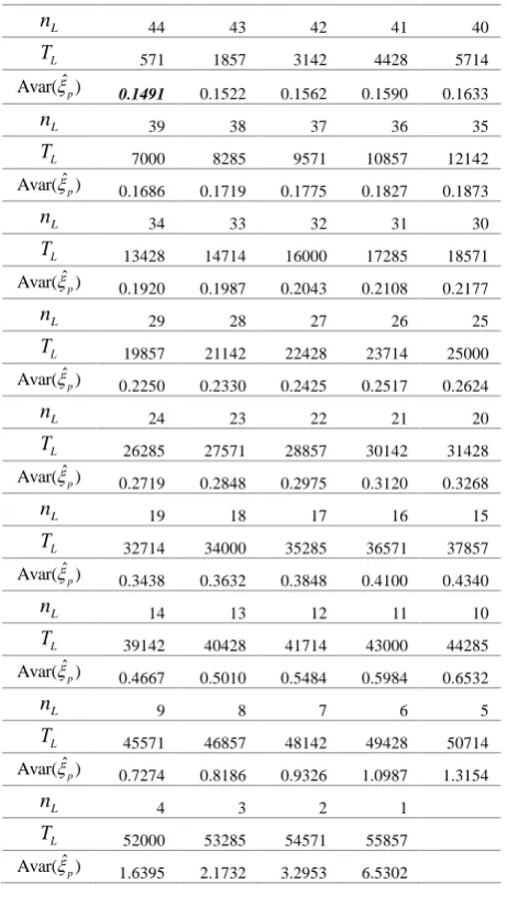
For life test, without the limitation of test time, under the total experimental cost constraint, enumeration method [8] is used to get the relationship between optimal test plan and reliability evaluation accuracy (asymptotic variance of ˆ

p  ), as shown in Table I.

[image:6.595.315.530.365.533.2]

(7)

failed before the test deadline is reached and the test does not need to continue. At this time, increasing the sample size and reducing the test time appropriately can obtain higher estimation accuracy.

Table I the asymptotic variance of ˆ p

 in life test

L

n ₄₄ ₄₃ ₄₂ ₄₁ ₄₀

L

T ₅₇₁ ₁₈₅₇ ₃₁₄₂ ₄₄₂₈ ₅₇₁₄

ˆ

Avar(p) 0.1491 0.1522 0.1562 0.1590 0.1633

L

n ₃₉ ₃₈ ₃₇ ₃₆ ₃₅

L

T ₇₀₀₀ ₈₂₈₅ ₉₅₇₁ ₁₀₈₅₇ ₁₂₁₄₂

ˆ

Avar(p) 0.1686 0.1719 0.1775 0.1827 0.1873

L

n ₃₄ ₃₃ ₃₂ ₃₁ ₃₀

L

T ₁₃₄₂₈ ₁₄₇₁₄ ₁₆₀₀₀ ₁₇₂₈₅ ₁₈₅₇₁

ˆ

Avar(p) 0.1920 0.1987 0.2043 0.2108 0.2177

L

n ₂₉ ₂₈ ₂₇ ₂₆ ₂₅

L

T ₁₉₈₅₇ ₂₁₁₄₂ ₂₂₄₂₈ ₂₃₇₁₄ ₂₅₀₀₀

ˆ

Avar(p) _0.2250 _0.2330 _0.2425 _0.2517 _0.2624

L

n ₂₄ ₂₃ ₂₂ ₂₁ ₂₀

L

T ₂₆₂₈₅ ₂₇₅₇₁ ₂₈₈₅₇ ₃₀₁₄₂ ₃₁₄₂₈

ˆ

Avar(p) 0.2719 0.2848 0.2975 0.3120 0.3268

L

n ₁₉ ₁₈ ₁₇ ₁₆ ₁₅

L

T ₃₂₇₁₄ ₃₄₀₀₀ ₃₅₂₈₅ ₃₆₅₇₁ ₃₇₈₅₇

ˆ

Avar(p) _0.3438 _0.3632 _0.3848 _0.4100 _0.4340

L

n ₁₄ ₁₃ ₁₂ ₁₁ ₁₀

L

T ₃₉₁₄₂ ₄₀₄₂₈ ₄₁₇₁₄ ₄₃₀₀₀ ₄₄₂₈₅

ˆ

Avar(p) 0.4667 0.5010 0.5484 0.5984 0.6532

L

n ₉ ₈ ₇ ₆ ₅

L

T ₄₅₅₇₁ ₄₆₈₅₇ ₄₈₁₄₂ ₄₉₄₂₈ ₅₀₇₁₄

ˆ

Avar(p) 0.7274 0.8186 0.9326 1.0987 1.3154

L

n ₄ ₃ ₂ ₁

L

T ₅₂₀₀₀ ₅₃₂₈₅ ₅₄₅₇₁ ₅₅₈₅₇

ˆ

Avar(p) _1.6395 _2.1732 _3.2953 _6.5302

VI. CONCLUSION

In this paper, for the Wiener degenerate failure products and two cases which are without and with measurement error in the degradation test, the reliability modeling methods with different number of measurement have been studied respectively. And we compare the effectiveness of life test and degradation test on reliability assessment. The research shows that:

(1) For the reliability evaluation based on the degradation test, it is necessary to make a reasonable analysis and determination of the factors affecting the test. For example, if there is no measurement error in the test, using the evaluation method for measurement error case will reduce accuracy. If the destructive measurement is used or each sample only measure once, different measurement times are required for each sample so as to identify the measurement error and the diffusion parameter.

(2) For the optimization of degradation test, the effects of measurement errors must be considered. Specifically, the measurement error has different influence on the accuracy of different model parameter. For example, the standard error of

MLE of drift parameter increases linearly with the measurement error, while the estimation accuracy of the diffusion parameter decreases nonlinearly when the measurement error increases.

(3) Degradation tests have significant advantages for reliability assessment compared to life tests. As far as we know, this paper is the first to quantitatively compare the degradation test and the life test. The results can be of practical significance for the study of reliability evaluation test optimization.

ACKNOWLEDGMENT

My deepest gratitude goes first and foremost to National Natural Science Foundation of China and commissioner of this activity. With financial support, I have this opportunity to communicate with other researcher all over the world. Secondly, I owe my sincere gratitude to my friends and my fellow classmates who gave me their help and time in listening to me and helping me work out my problems during the difficult course of the thesis. Last my thanks would go to my beloved family for their loving considerations and great confidence in me all through these years.

REFERENCES

[1] Lawless, J. F.. Statistical Models and Methods for Lifetime Data[M]. John Wiley, New York.1982,293-294

[2] C.J. Lu and W, Q. Meeker, Using degradation measures to estimate a time-to-failure distribution[J]. Tech-nometrics vol. 35(2), 1993:161-174.

[3] C. Joseph Lu, William Q. Meeker, Luis A. Escobar. A comparison of degradation and failure-time analysis methods for estimating a time-to-failure distribution[J]. Statistica Sinica, 1996, 6(3):531-546. [4] Chhikara, R.S.,Folks, J.L.. The Inverse Gaussian Distribution as a

Lifetime Model.[J], 1977,19(4):461.

[5] Jun-mei Jia, Zai-zai Yan, Xiu-yun Peng. Estimation for inverse Gaussian Distribution Under First-failure Progressive Hybird Censored Samples[J]. Filomat 31:18(2017):5743–5752.

[6] G. A. Whitmore. Estimating degradation by a wiener diffusion process subject to measurement error[J],1995,1(3):307-319.

[7] Marseguerra M, Zio E. Designing Optimal Degradation Tests via Multi-Objective Genetic Algorithms[J]. Reliability Engineering and System Safety, 2003(79):87-94.

[8] Tang L C, Yang G Y, Xie M. Planning of Step-Stress Accelerated Degradation Test[C]. RAMS, 2004:287-292.

[9] Liao C M, Tseng S T. Optimal Design for Step-Stress Accelerated Degradation Tests[J]. IEEE Transactions on Reliability. 2006(55):59-66.

[image:7.595.54.285.115.527.2]