A Novel Ensemble Learning Approach to Unsupervised Record
Linkage
Anna Jurek, Jun Hong, Yuan Chi, Weiru Liu
PII:
S0306-4379(16)30506-3
DOI:
10.1016/j.is.2017.06.006
Reference:
IS 1228
To appear in:
Information Systems
Received date:
21 October 2016
Revised date:
25 June 2017
Accepted date:
27 June 2017
Please cite this article as: Anna Jurek, Jun Hong, Yuan Chi, Weiru Liu, A Novel Ensemble Learning
Approach to Unsupervised Record Linkage,
Information Systems
(2017), doi:
10.1016/j.is.2017.06.006
ACCEPTED MANUSCRIPT
Highlights• A novel unsupervised approach to record linkage has been proposed
• The approach combines ensemble learning and automatic self learning
• An ensemble of diverse self learning models is generated through applica-tion of different string similarity metrics schemes
• Application of ensemble learning alleviates the problem of having to select the most suitable similarity metric scheme and improves the performance
of an individual self learning model
ACCEPTED MANUSCRIPT
A Novel Ensemble Learning Approach to Unsupervised
Record Linkage
Anna Jureka, Jun Hongb, Yuan Chia, Weiru Liuc
aSchool of Electronics, Electrical Engineering and Computer Science, Queen’s University
Belfast, Computer Science Building, 18 Malone Road, BT9 5BN Belfast, United Kingdom bDepartment of Computer Science and Creative Technologies, University of the West of
England, Coldharbour Lane, BS16 1QY Bristol, United Kingdom
cMerchant Venturers School of Engineering, University of Bristol,75 Woodland Road, BS8
1UB Bristol, United Kingdom
Abstract
Record linkage is a process of identifying records that refer to the same
real-world entity. Many existing approaches to record linkage apply supervised
ma-chine learning techniques to generate a classification model that classifies a pair
of records as either match or non-match. The main requirement of such an
approach is a labelled training dataset. In many real-world applications no
labelled dataset is available hence manual labelling is required to create a
suffi-ciently sized training dataset for a supervised machine learning algorithm.
Semi-supervised machine learning techniques, such as self-learning or active learning,
which require only a small manually labelled training dataset have been applied
to record linkage. These techniques reduce the requirement on the manual
la-belling of the training dataset. However, they have yet to achieve a level of
accuracy similar to that of supervised learning techniques. In this paper we
propose a new approach to unsupervised record linkage based on a combination
of ensemble learning and enhanced automatic self-learning. In the proposed
approach an ensemble of automatic self-learning models is generated with
dif-ferent similarity measure schemes. In order to further improve the automatic
self-learning process we incorporate field weighting into the automatic seed
selec-tion for each of the self-learning models. We propose an unsupervised diversity
measure to ensure that there is high diversity among the selected self-learning
mod-ACCEPTED MANUSCRIPT
els to remove those with poor accuracy from the ensemble. We have evaluated
our approach on 4 publicly available datasets which are commonly used in the
record linkage community. Our experimental results show that our proposed
approach has advantages over the state-of-the-art semi-supervised and
unsuper-vised record linkage techniques. In 3 out of 4 datasets it also achieves comparable
results to those of the supervised approaches.
Keywords: Unsupervised record linkage, data matching, classification,
ensemble learning
1. Introduction
Record linkage (RL), also referred to as data matching or entity resolution,
is a process of finding records that correspond to the same entity from one or
more data source [1]. Given two data sources, each pair of records from the
data sources can be classified into one of two classes: match and non-match.
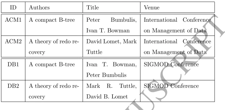
Table 1 shows a simple example of RL. The table contains records from two
bibliographic data sources (DBLP, ACM digital library). The aim is to
iden-tify those pairs of records referring to the same publications, which in this case
are (ACM1, DB1) and (ACM2, DB2). Any other pairs of records should be
identified as non-match. RL has been widely applied in data management,
data warehousing, business intelligence, historical data collection and medical
research [2]. If records have error-free and unique identifiers, such as social
se-curity numbers, RL is a straightforward process that can be easily performed by
the standard database join operation. In many cases, however, such a unique
identifier does not exist and the linkage process needs to be performed by
match-ing the correspondmatch-ing fields of two records. A lot of efforts have been made to
develop techniques for RL [3]. Unfortunately, in many cases the same data can
be represented in different ways in different data sources due to factors such
as different conventions (e.g., International Conference on Management of Data
versus SIGMOD Conference). Furthermore, data quality is often affected by
ACCEPTED MANUSCRIPT
Table 1: An Example of RL.
ID Authors Title Venue
ACM1 A compact B-tree Peter Bumbulis,
Ivan T. Bowman
International Conference
on Management of Data
ACM2 A theory of redo
re-covery
David Lomet, Mark
Tuttle
International Conference
on Management of Data
DB1 A compact B-tree Ivan T. Bowman,
Peter Bumbulis
SIGMOD Conference
DB2 A theory of redo
re-covery
Mark R. Tuttle,
David B. Lomet
SIGMOD Conference
not always the case that records referring to the same entity have the same
values on the corresponding fields. Therefore, sophisticated RL techniques are
required in order to identify records that refer to the same real-world entity.
Existing RL methods rely strongly on use of similarity measure, in which
selection of such measures is a key issue [3]. There are many of available
simi-larity measures, e.g., Edit Distance, Jaro and Smith-Waterman [3]. Depending
on the types of data in RL, similarity measures have different levels of accuracy
[4].
Linking two large datasets could be computationally expensive. If we need to
link two datasets,AandB, then potentially we should compare each record from
Awith each record fromB. Hence, the total number of comparisons would be
|A|×|B|. To reduce the potentially large number of record comparisons different forms of indexing and filtering, collectively referred to as blocking [5], [6], are
deployed in RL systems. The idea of blocking is to use a blocking function to
divide records into a set of blocks. The candidate pairs of records for linkage are
then selected from records in the same block only. The existing approaches to
RL can be broadly divided into two categories. The first category of approaches
rely on applying generic rules and similarity measures to identify those pairs
ACCEPTED MANUSCRIPT
of approaches rely on a training dataset to train a classification model using
appropriate statistical and machine learning techniques. In these techniques,
each pair of records is represented as a similarity vector withN elements. The
similarity vector represents a set ofNnumeric similarities, each calculated with
a similarity measure on the corresponding pair of field values of the two records.
The task of RL is then considered as a similarity vector classification problem
[9], i.e., whether a similarity vector is classified as match or non-match, for a
pair of matching or non-matching records respectively.
The main limitation of the second category of approaches is that they require
a labelled training dataset. In many real world situations no labelled dataset is
available. In addition, given the sensitivity of the data in RL, very often it is
not possible to manually label the records [10]. Therefore, there is a big need
for fully unsupervised RL models. To meet this challenge we propose a new
approach to RL, which does not require any labelled dataset. The proposed
ap-proach combines ensemble learning [11] and automatic self-learning techniques
[12]. With self-learning [13] a supervised learning algorithm is trained on a
small set of labelled records (seeds) to generate an initial classification model.
The initial classifier is then applied to unlabelled records in order to
gener-ate more labelled records for the supervised learning algorithm. Only those
records that the classifier is most certain about are labelled and added into
the training dataset. The updated training dataset is further used to generate
another classifier. This process iterates until all unlabelled records have been
labelled with the final classifier generated. When there is no labelled record
readily available for training the initial classifier, a small set of records needs to
be selected and labelled automatically (automatic seed selection). It has been
shown that self-learning can outperform other unsupervised algorithms, such as
Expectation-Maximization [13]. Self-learning with automatic seed selection has
been already investigated in RL and promising results have been achieved [12].
The goal of ensemble learning [11], [14] is to train and combine a number of
different classification models to obtain better performance than any of those
ACCEPTED MANUSCRIPT
to as a classifier ensemble. Classification models included in an ensemble are
commonly refereed to as base classifiers (BCs). Ensemble learning has been
shown to improve the performance of classification algorithms, such as SVM
[15], Decision Tree [16] and Nearest-Neighbor [17]. The key objective in
ensem-ble learning is to train a set of highly diverse base classifiers. Two classification
models are considered highly diverse if they make mistakes on (misclassify)
dif-ferent groups of instances. It has been shown that combining classifiers with
low diversity does not improve classification accuracy [18]. One approach to
training a collection of diverse classification models is to use a different
(ran-domly selected) subset of the training dataset to train each of the classifiers
(Bagging) [19]. Classifiers trained on different datasets are expected to make
different classification decisions. An alternative is to, instead of randomly
sam-pling from the training dataset, randomly select features, like in the case of
Random Forest [20]. With Random Forest, each of the BC is trained with a
different subset of features. With another technique, referred to as Boosting
[21], the weights of the instances from the training set are dynamically altered
based on the accuracy of the classifier. After a BC is built and added to the
ensemble, all instances are re-weighted: those that have been correctly or
incor-rectly classified lose or gain weights respectively. The modified distribution of
the training dataset is taken under consideration in the training process of the
next BC. Any supervised classification learning algorithm can be applied with
the aforementioned techniques to generate the base classifiers. The goal of all
the ensemble techniques is to construct a multitude of BCs at training time and
output the class that is the mode of their individual predictions at
classifica-tion time. Very often only a subset of BCs is selected in order to increase the
diversity of the ensemble. A common practice is to measure diversity among a
group of BCs and select a group of classifiers with the highest diversity to form
an ensemble [22]. A number of methods for measuring the diversity among the
BCs in an ensemble have been proposed, including pairwise and non-pairwise
diversity measures [23]. Pairwise diversity measures are defined for a pair of
ACCEPTED MANUSCRIPT
diversity values. Non-pairwise diversity measures are defined on the ensemble
as a whole.
Our proposed approach incorporates ensemble learning and self-learning
techniques into RL. Self-learning with automatic seed selection addresses the
problem of lack of labelled datasets. However, it has yet to achieve a level of
accuracy similar to that of supervised learning techniques [12]. Another issue
with the unsupervised models for RL is related to the selection of an appropriate
similarity measure used for generating similarity vectors. The performance of
the RL algorithms relies strongly on the selected similarity measure [4]. It is,
however, difficult to select an appropriate similarity measure without labelled
datasets [24]. With our proposed approach we generate an ensemble of diverse
self-learning models by applying different combinations of similarity measure.
By using different combinations of similarity measures we can generate
differ-ent sets of similarity vectors that can be used to generate differdiffer-ent self-learning
models. To ensure high diversity among the self-learning models we apply the
proposed seed Q-statistic diversity measure. We also propose to use
Contribu-tion Ratios of BCs to eliminate those with very poor accuracy from the final
ensemble.
In this paper we make the following contributions: (1) We propose a
frame-work for unsupervised RL, which incorporates ensemble learning and self-learning
into RL. (2) We improve the existing automatic self-learning technique for RL
[12] by incorporating unsupervised field weighting into the process of automatic
selection of seeds. (3) We propose an ensemble learning method based on the
selection of different similarity measure schemes. This alleviates the problem
of having to select the most suitable similarity measure scheme and improves
the performance of an individual classifier. (3) We propose a new unsupervised
diversity measure, which ensures high diversity among the self-learning models.
(4) We propose to use the contribution ratios of BCs to eliminate the weakest
ACCEPTED MANUSCRIPT
2. Related WorkGiven the importance and challenges of RL, there has been strong interest
in the last decade and significant progress has been made in this field [25][26].
In order to address the problem of lack of labelled data various semi-supervised
learning techniques have been proposed for RL over the past few years. In
semi-supervised learning only a small set of labelled instances and a large set
of unlabelled instances are used in the training process. A popular approach
to semi-supervised RL is referred to as active learning (AL) [27]. AL identifies
highly informative instances for manual labelling that are later used for training
classification models. In [28] the most informative instances are selected for
manual labelling based on the classifications by a group of classifiers. The
instances that are not assigned to the same class by majority of the classifiers
are selected for manual labelling. In [29] a set of similarity vectors are ranked
and those in the middle (fuzzy) region are selected for manual labelling. The
labelled instances are further used to train a classification model.
An interactive training model based on AL is proposed in [30]. In this
approach all the record pairs are clustered by their similarity vectors. A number
of similarity vectors from each cluster are selected and their corresponding pairs
of records are selected for manual labelling. If all selected pairs of records from
a cluster are labelled as match, then the remaining similarity vectors from the
cluster are automatically labelled as match and added to the training dataset.
Similarly, if all selected pairs of records from a cluster are labelled as non-match,
the remaining similarity vectors in the cluster are automatically labelled as
non-match and included in the training dataset. If the selected pairs of records from
a cluster belong to different classes then the cluster is further split into
sub-clusters. The process is repeated recursively until all the pairs of records are
added to the training dataset.
A different semi-supervised learning based approach to RL is proposed in
[31]. The system takes as input a small set of training examples, referred to as
ACCEPTED MANUSCRIPT
is then applied to classify the unseen data. A small percentage of the most
con-fidently classified record pairs are selected to iteratively train the classification
model. The process is repeated for a number of iterations or until all the unseen
data are labelled. To maximize the performance of the model on unseen data an
ensemble technique referred to as boosting is employed together with weighted
Majority Voting. Random Forest and Multilayer Perceptrons are applied as the
BCs in the ensemble. The proposed system requires a number of parameters to
be specified, including the maximum number of iterations, the percentages of
the most confident matching and non-matching examples to be selected in each
iteration.
Semi-supervised learning significantly reduces the number of manually
la-belled examples required for generating a classification model. However, it still
requires a certain amount of human input in the training process. In [9] two
unsupervised RL methods were proposed. The first one, referred to as
Clus-tering Record Linkage Model, uses k-means clustering to divide all similarity
vectors into three clusters. Depending on the values in the similarity vectors,
each cluster is labelled with one of the three matching status, match, non-match
and possibly match. The similarity vectors in the first two clusters were
auto-matically labelled, while the third cluster required manual labelling. With the
second method, referred to as Hybrid Record Linkage Model, the RL process
consists of two steps. First, clustering is used to predict the matching status
of a small set of similarity vectors. In the second step, the labelled similarity
vectors are used as training set for a supervised learning algorithm.
In [12] an unsupervised approach to RL based on automatic self-learning
is proposed. In this work an approach to automatic seed selection referred to
as nearest based was applied. With the nearest based approach, all similarity
vectors are sorted by their distances (e.g., Manhattan or Euclidean distance)
from the origin [0,0, . . .] and from the vector with all similarities equal to 1
([1,1, . . .]). Following this, the respective nearest vectors are selected as match
and non-match seeds. The numbers of match and non-match seeds to be selected
ACCEPTED MANUSCRIPT
of the non-match seeds, namely 1%, 5% and 10% of the entire dataset. Following
this, an appropriate ratio of similarity vectors was selected as match seeds. After
selecting seeds, a classification model is trained incrementally as with the
self-learning technique. In the same work it was observed that this approach did
not provide good quality match seeds when the dataset contained only a small
number of matching records or there were some fields with a large proportion
of abbreviations.
In more recent work unsupervised techniques for RL based on maximizing
the value of pseudoF-measure [32] were proposed [32], [33]. PseudoF-measure
is formulated based on the assumption that while different records often
repre-sent the same entity in different repositories, distinct record within one dataset
is expected to denote distinct entity. It can be calculated using sets of unlabelled
records. The idea is to find the decision rule for record matching which
maxi-mizes the value of the objective function (pseudoF-measure) applying genetic
programming [32] or a hierarchical grid search [33]. The RL rules are
formu-lated by manipulating weights and similarity measures for pairs of attributes,
modifying the similarity threshold value and changing the aggregation function
for individual similarities. To the best of our knowledge, the approaches based
on the application of the pseudoF-measure are the state-of-the-art in the area
of unsupervised RL.
It can be noted that, apart from the method presented in [12], [32], [33],
in each of the aforementioned methods some level of human input is required.
These methods are not applicable in many real-world situations. In particular
for privacy preserving RL, where the data is private and confidential [10], it
may be impossible to label the data manually. The method proposed in [12]
does not require any labelled data, however, it performs significantly worse than
supervised methods. At the same time a recent study found that on real data
the pseudo F-measure is often negatively correlated with the trueF-measure
[33], which raises concerns about whether currently defined pseudoF-measure
ACCEPTED MANUSCRIPT
3. Preliminary and Problem FormulationGiven two sets of recordsR1and R2, RL is defined as a task of identifying
pairs of records (r1, r2)∈R1×R2that refer to the same entity (e.g., a person).
The decision whether a pair of records represent a match is based on the
simi-larity between the two records on each of their fields, which can be determined
with a similarity measure.
Definition 3.1. (Similarity measure) Given two records r1and r2 represented
byN fieldsf1, . . . , fN, a similarity measuremquantifies similarity between the
two records on one of the fields. It returns a numeric value ranging between0
and1, referred to as a similarity value. A similarity measure is represented as
m(r1.fi, r2.fi)wherer1.fi andr2.fi represent the values of fieldfi in recordsr1
andr2 respectively.
Value 1 indicates that the pair of records have the exact same values on a filed
according to the similarity measure. Value 0 indicates that there is no similarity
between the filed values for the two records. An example similarity measure
could be Edit distance which for given two strings (e.g.,surnames) determines
the minimum number of operations that are required to transform one string
into the other. For a pair or records represented by N fields a combination of
N different similarity measure can be applied to determine similarity between
the records on each of theN fields.
Definition 3.2. (Similarity measure scheme). Given two records r1 and r2
represented by N fields f1, . . . , fN, a similarity measure scheme is defined as
Sc = m1, . . . , mN, where mi represents a similarity measure used to measure
the similarity betweenr1 andr2 on fieldfi, fori= 1, . . . , N.
Following the application of a similarity measure scheme, for each pair of records
with N fields we can construct aN-dimensional vector representing similarity
values between the records on the fields.
Definition 3.3. (Similarity vector). Given two recordsr1 and r2 represented
ACCEPTED MANUSCRIPT
similarity vector for r1 andr2 is defined as:
−−−−−−−−→
(Sc(r1, r2)) =< m1(r1.f1, r2.f1), . . . , mN(r1.fN, r2.fN)> (1)
The aim of RL process is to classify each similarity vector into one of two classes:
matches (M) and non-matches (U). The goal of our work is to develop a learning
algorithm, which, given two sets of records R1 and R2 and a set of available
similarity measuresM, can be used to construct a model for classifying a pair
of records as match or non-match. The classification model should be trained
without requiring any manually labelled data as input.
The general idea of our proposed approach is to generate an ensemble of
self-learning classifiers using different similarity measure schemes. Self-learning
is an approach to semi-supervised learning where small amount of labelled data
and large amount of unlabelled data are used for training.
Definition 3.4. (Self-learning). Given training dataset L = {xi, yi}li=1
(ref-ereed to as seeds) and unlabelled datasetU ={xj}lj+=ul+1 (usually LU), the
self-learning process aims to train a classifier hon L initially and then use the
classifier to label all unlabelled data in U. Following this, the most confidently
classified unlabelled examples are selected as new training examples and moved
into L. The process is repeated until a stopping condition is met.
One may notice a major difference between self-learning and the
aforemen-tioned active learning. Instead of choosing the most confident examples to be
labelled by itself, active learning actively selects the most problematic examples
from the unlabelled dataset and asks these examples to be manually labelled.
With the proposed approach a number of different similarity measure schemes
are selected. Each of the selected similarity measure schemes is used to generate
a different set of similarity vectors. Each set of similarity vectors is then used
to generate a different self-learning classifier. To a certain extent, our ensemble
method is based on a similar principle to Bagging. With Bagging, each BC is
trained with different (randomly selected) subset of the training dataset.
ACCEPTED MANUSCRIPT
training datasets using a set of different similarity measure schemes. As it is
the case in Bagging, with the proposed approach all BCs are trained with the
same learning algorithm but with different training datasets.
4. Proposed Approach
Figure 1 shows our proposed RL framework. Two sets of unlabelled records
are provided as input. The RL process is performed in six steps. As with
a typical RL approach, blocking is the first step and it can be thought of as
a pre-processing step. We investigated two techniques, a standard blocking
method referred to as canopy clustering [5] and a recently proposed unsupervised
blocking scheme learner for blocking [34]. Better reduction ratio of the record
pairs was obtain with the latter technique therefore we used it in our paper. To
our best knowledge, this is the state-of-the-art method for unsupervised blocking
in RL. It is relatively easy to implement and performs well empirically. The
blocking method is divided into two phases. First, a weakly labelled dataset is
generated automatically. In the second phase the problem of learning a blocking
scheme from the weakly labelled dataset is cast as a Fisher feature selection
problem [35].
The second step of the RL process is the selection of similarity measure
schemes. In this step we search the whole space of all possible similarity measure
schemes in order to select the most diverse subset of it. In the third step (seed
selection with field weighting) each of the selected similarity measure schemes
is first used to generate a set of similarity vectors. Then the automatic seed
selection process is performed on each set of similarity vectors. As the output
of this step different sets of seeds are selected. In the fourth step (Selecting
the most diverse sets of seeds), the diversity between sets of seeds is measured
using the proposed technique referred to as SeedQStatistics. Only those most
diverse sets of seeds are selected. In the fifth step the self-learning algorithm
is applied with each of the selected sets of seeds. In the last step the proposed
ACCEPTED MANUSCRIPT
ensemble. Finally, for each pair of records the mode of the predictions of the
selected self-learning models is provided as the final prediction. Each of the
aforementioned steps is described in detail in the following sections.
Generating pool of similarity schemes
Similarity metrics:
𝐷 = 𝑑1, … , 𝑑𝑀
Generating similarity vectors with each similarity scheme Selecting seeds for
each set of similarity vectors
Final Classification Selecting sets of
seeds with the highest diversity
Self learning with the selected sets of
seeds
Selecting the final ensemble using the Contribution Ratio
Records A
Records B
Blocking
Record Pairs
Step 1: Blocking Step 2: Similarity schemes selection
Step 3: Seed selection with fields weighting Step 4: Selecting diverse set of
seeds
Step 5: Self-learning Step 6: Selecting BCs for final ensemble
Figure 1: RL process with the proposed approach.
4.1. Selecting similarity measure schemes
For a given set of M similarity measures we could construct MN possible
similarity measure schemes of sizeN, whereNis the number of fields. However,
whenM andN are large numbers, it would be infeasible to learn all BCs using
each of the possible similarity measure schemes. In addition, the key of ensemble
learning is to combine a set of diverse BCs. We need to select those similarity
measure schemes that produce the most diverse sets of similarity vectors from
the given dataset. We propose a method for selecting such a pool of similarity
measure schemes. We first select a set of similarity measure for each of the
ACCEPTED MANUSCRIPT
product of the sets of similarity measure selected for each of the fields. In order
to select a set of similarity measure for fieldf, in which no similarity measure is
too similar to another, we define the similarity between two similarity measure.
Definition 4.1. (Field similarity between records) Given a similarity measure
m and a pair of records r1 and r2, each with N fields, f1, . . . , fN, the field
similarity between r1 and r2 on field fi, for i = 1,2, . . . , N, is defined as:
m(r1.fi, r2.fi).
Definition 4.2. (Similarity between Similarity Measures) For a given set of
records R and two similarity measuresm1 and m2, let −−−−−−→m1(R, f)and −−−−−−→m2(R, f)
be two vectors with each corresponding pair of elements in−−−−−−→m1(R, f)and−−−−−−→m2(R, f)
representing the field similarity between each possible pair of records inRon field
f. The similarity betweenmi andmj on field f is defined as:
simf(mi, mj) =cossim(−−−−−−→mi(R, f),−−−−−−→mj(R, f)) (2)
Cosine similarity [36] measures the similarity between two vectors of an inner
product space by the cosine of the angle between them. We aim to select a set
of similarity measures for each of the fields, in which no cossim between two
similarity measures is greater than a threshold.
The selection method is described in Algorithm 1. It takes as input a set of
similarity measures, a set of records and parameterp. The parameter indicates
the similarity threshold, i.e., the maximum similarity that two measures selected
for the same field can have. The method selects a subset of similarity measures ˇ
Vf for each fieldf. The setVf refers to all the similarity measures provided as
input. In the first step a pair of similarity measures from Vf with the lowest
similarity on f is selected and moved to ˇVf (line 3). The remaining of the
process is performed in iterations. First, we remove all similarity measures from
Vfthat have similarity onfhigher thanpwith any of the similarity measures in
ˇ
Vf (Line 5). Following this, in lines 6-7 we select a similarity measures fromVf
which has the highest similarity onf with any of the measures from ˇVfand move
ACCEPTED MANUSCRIPT
last step, a pool of similarity measure schemes is generated as a cross product
of the similarity measures selected for each of the fields (line 10). The value
of parameter p influences the number of similarity measures selected for each
field and consequently the number of similarity measure schemes selected. The
higher the value of p, the more similarity measure schemes will be generated.
For p = 1, the number of similarity measure schemes will be MN. If the run
time of each similarity measure is bounded above byO(c) then for P pairs of
records represented byNfields the process of generating similarity vectors with
one scheme should takeO(N×P×c). With our proposed approach the run time
will beO(s×N×P×c) wheresis the number of selected similarity schemes.
Algorithm 1 Generating a pool of similarity measure schemes
Input: ψ=m1, . . . , mM: a set of similarity measures,R: a set of records each
withN fieldsf1, . . . , fN,p∈(0,1): similarity threshold
Output: Cˇ: a set of similarity measures schemes
1: for allf ∈F do
2: Vf=m1, . . . , mM, ˇVf =∅
3: Select a pair of similarity measures fromVfwith the lowest similarity and
move them to ˇVf
4: whileVf6=∅do
5: Remove everymfromVf such that argmaxmi∈Vˇfsimf(mi, m)> p
6: Selectm∈Vf wherem= argmaxmj∈Vfargmaxmi∈Vˇfsimf(mi, mj)
7: MovemfromVf to ˇVf
8: end while
9: end for
10: returnCˇ = ˇV1× · · · ×VˇN
Theorem 4.1. Let ψ be a set of similarity measures and C¨ be a set of all
possible similarity measure schemes generated from ψ for a set of records R.
ACCEPTED MANUSCRIPT
following is true:
∀Ci∈C¨ ∃Cj∈Cˇ ∀fn∈F simfn(m i
n, mjn)≥p (3)
whereCi=mi1, . . . , min,Cj=mj1, . . . , mjnandpis the similarity threshold given
as an input.
Theorem 4.1 claims that the selection method presented in Algorithm 1
generates a pool of similarity measure schemes that covers a space of similarity
measure schemes with the level of similarity equal to p. This means that for
any similarity measure scheme Ci we can find a similarity measure scheme Cj
from the selected pool, such that any corresponding pair ofmi andmjfromCi
andCj have similarity higher thanp(sim(Ci, Cj)> p).
Proof. Following Algorithm 1 ˇCis generated as a cross product ˇC = ˇV1×, . . . ,×VˇN.
LetCi=< mi1, . . . , miN > be a similarity measure scheme selected from ¨C. We
show that there exists Cj ∈ Cˇ such that sim(Ci, Cj) > p. We consider the
following two scenarios:
I.Ci∈Cˇ then ∀fn∈F simn(min, mjn) = 1> p
II.Ci∈Cˇ
LetCj ∈Cˇ be as follows:
Cj=< mj1, . . . , m
j N >:m
j n=
mi
n ifmin∈Vˇn
argmaxm∈Vˇnsimfn ifm i n∈/Vˇn
Ifmi
n∈Vˇn thensimn(min, mjn) = 1> p. Otherwise we have:
mni ∈/Vˇn =⇒ ∃m∈Vˇn sim(m, min)> p =⇒ max m∈Vˇn
sim(m, min)> p
Finally we have the following.
∀fn∈F simfn(m i
ACCEPTED MANUSCRIPT
4.2. Seed selection with field weighting
Each of the selected similarity measure schemes is used to generate a set of
similarity vectors for all the pairs of records produced by the blocking algorithm.
For each vector set, a small group of similarity vectors are automatically labelled
as match and non-match, which will be used as seeds in the self-learning method.
4.2.1. Field weighting
In this paper we propose an improvement to the approach, proposed in [12],
to automatic seed selection for self-learning. In the original approach in [12]
those similarity vectors that are the nearest to the perfect match and perfect
non-match as the seeds.
Definition 4.3. (Perfect Match). A perfect match is a similarity vector, with
each of its elements having a similarity value of 1, that is,
− →1 =< x
i>i=1,...,n,∀i xi= 1 (4)
which indicates that the pair of records represented by the similarity vector has
the same value on each of their corresponding fields.
Definition 4.4. 5 (Perfect Non-Match). A perfect non-match is a similarity
vector, with each of its elements having a similarity value of 0, that is,
− →0 =< x
i>i=1,...,n,∀i xi= 0 (5)
which indicates that the pair of records represented by the similarity vector has
completely different values on each of their corresponding fields.
In our improved approach we still select similarity vectors nearest to the
perfect match and perfect non-match. However, we take into account the
dis-tinguishing power of fields when calculating the distance between a similarity
vector and the perfect match or non-match. It is known that some fields may
be more distinguishing than the others in the RL process [37]. For example,
the fieldlast name is more distinguishing than the fieldf irst namegiven that
ACCEPTED MANUSCRIPT
the distinguishing power of a field. We say that a field has high distinguishing
power if the similarity between any pair of records on the field is close to 1 when
the records match and 0 otherwise.
Definition 4.5. (Distinguishing Power of a Field) For a set of similarity vectors
labelled as match (XM)and non-match(XU), the distinguishing power of field
fj is defined as:
dpfj = P
x∈XM
xj+ P x∈XU
(1−xj)
|XM|+|XU| (6)
wherexj represents the value of fieldj in similarity vectorx.
The numerator sums up the distances between each similarity vector from
XM and −→0 and each similarity vector fromXU and−→1 onf
j. Thedpfj is the
average of such distances among all vectors inXM orXU. It equals to 1 if all
the matches have a similarity value of 1 onfj, and all the non-matches have a
similarity value of 0 onfj. In such a case, fieldfjhas the highest distinguishing
power for the given dataset.
Our intention is to assign a weight to each field in proportion to its
distin-guishing power. The weights are then used for calculating the distance between
a similarity vector and either the perfect match or the perfect non-match in
the seed selection process. Given that our proposed method is fully
unsuper-vised and we do not have any labelled data we are not able to calculate the
distinguishing power of a field as described in Definition 4.5. For this reason
we instead use an unsupervised field weighting method that was proposed for
the k-means clustering algorithm in [38]. We are able to show (Theorem 4.2)
that the weight assigned to a field with this method is in proportion to the
distinguishing power of the field.
The method in [38] first clusters the unlabelled records using the k-means
algorithm. Then, a weight is assigned to each field based on the sum of within
cluster distances of the field. Each of the within cluster distances for a field
represents the difference on this field between the centroid of the cluster and
ACCEPTED MANUSCRIPT
a field with a lower sum of the within cluster distances. The weights are then
used in the clustering process in the next iterations. The process iterates until
there is no change to any of the weights. It has been shown in [38] that the
weights of fields reflect their levels of significance.
In our work we follow the same principle as in [38] with two specific clusters
representing two sets of seeds, one containing the match seeds (XM with the
perfect match as the centroid) and another containing the non-match seeds
(XU with the perfect non-match as the centroid). After the two sets of seeds
are selected the weights of fields are calculated as follows:
ωj= 1
|{fi:Di=0}| ,if Dj= 0,
0 ,if Dj6= 0∧ |{fi6=j:Di= 0}| 6= 0,
1
n
P
k=1
(Dj/Dk)
,otherwise.
(7)
The Dj is the sum of all the distances between every vector in XM and the
perfect match, and every vector in XU and the perfect non-match on fieldf j
for j = 1. . . n. It can be seen from Definition 4.5 that, if Dj = 0 then the
distinguishing power of fj is 1. Therefore, if there are any fields with Dj = 0
(condition 1) they are assigned with equal weights and the remaining fields
have a weight of 0 (condition 2) and are not taken under consideration while
calculating the final similarity. If there is no field withDj= 0 then all the fields
are assigned with weights calculated using formula in condition 3. The weights
total to 1 (Theorem 4.3).
Theorem 4.2 states that the weight of a field calculated with Formula 7 is
proportional to the distinguishing power of the field.
Theorem 4.2. For a set of similarity vectors, each labelled as either match
(XM)or non-match(XU), for any two fieldsf
i andfj we have:
ωi≤ωj⇔dpfi< dpfj (8)
Proof. First we show that the theorem holds if|{fi:Di = 0}| 6= 0. According
ACCEPTED MANUSCRIPT
fieldfj is equal to either 0 (ifDj6= 0) or |{fi:D1i=0}| (ifDj= 0). Obviously 0<
1
|{fi:Di=0}| and according to Definition 4.5, fields withDj = 0 have the highest
distinguishing power. Therefore: dpfj:Dj=06 < dpfi:Di=0 so the theorem holds.
Below we demonstrate that the theorem also holds when|{fi:Di= 0}|= 0.
ωi< ωj⇒ Pn 1
k=1 Di/Dk
< Pn 1
k=1 Dj/Dk
⇒
n X
k=1
Di/Dk > n X
k=1
Dj/Dk⇒
Di> Dj⇒ X
x∈XM
(1−xi) + X
x∈XU
xi> X
x∈XM
(1−xj) + X
x∈XU
xj ⇒
X
x∈XM
1− X
x∈XM
xi+ X
x∈XU
xi> X
x∈XM
1− X
x∈XM
xj+ X
x∈XU
xj⇒
− X
x∈XM
xi+ X
x∈XU
xi>− X
x∈XM
xj+ X
x∈XU
xj⇒
− X
x∈XU
1− X
x∈XM
xi+ X
x∈XU
xi>− X
x∈XU
1− X
x∈XM
xj+ X
x∈XU
xj⇒
X
x∈XU
1 + X
x∈XM
xi− X
x∈XU
xi< X
x∈XU
1 + X
x∈XM
xj− X
x∈XU
xj⇒
X
x∈XM
xi− X
x∈XU
(1−xi)< X
x∈XM
xj− X
x∈XU
(1−xj)⇒
P
x∈XM
xi− P x∈XU
(1−xi)
|XM∪XU| < P
x∈XM
xj− P x∈XU
(1−xj)
|XM∪XU| ⇒dpfi< dpfj
The implicationdpfi < dpfj →ωi< ωj can be proved accordingly.
Theorem 4.3. Pni=0 ωi= 1.
Proof. If there is at least one fieldfisuch asDi= 0 then the weights of all the
files with Di = 0 are the same and add up to 1 so the theorem holds. Let0s
assume that there are N fields f1, . . . , fN and ∀j=1...,NDj 6= 0. According to
Formula 7 we have:
ωj= N 1 P k=1
Dj/Dk
= 1
Dj/D1+· · ·+Dj/DN
ACCEPTED MANUSCRIPT
DenotingD1×· · ·×Di−1×Di+1×· · ·×DN by ¨D−iand bringing all the fractions
to the common denominator we get:
1
Dj
D1+· · ·+
Dj DN
=
QN
i=1Di
QN
i=1Di+Dj×Pi=1...n,i6=jD¨−i
=
= Dj×D¨−j
Dj×D¨−j+Dj×Pi=1...N,i6=jD¨−i
=
= ¨ D¨−j
D−j+Pi=1...N,i6=jD¨−i
= P D¨−j
i=1...nD¨−i
Consequently:
N X
j=1 ωj =
¨
D−1
PN
i=1D¨−i
+ · · · + PDN¨−N
i=1D¨−i
= D¨−1P+N· · ·+ ¨D−N
i=1D¨−i
= 1
4.2.2. Seed Selection
For a given set of similarity vectorsX, the seed selection process is performed
in two phases as illustrated in Figure 2. All the steps of the seed selection proces
are described in Algorithm 2. In the first phase, an initial set of similarity
vectors is selected using the given distance metric (dw) and two thresholds,
tM for match seeds and tU for non-match seeds (lines 4-11). In this paper
we use Manhattan distance. However, other distance metrics could also be
used. Initially both Manhattan and Euclidean distances were considered but
empirically Manhattan distance worked slightly better. At the beginning all
the field weights have the same values. The minimum numbers of similarity
vectors to be selected initially as match and non-match seeds are specified by
two parameters,mM andmU (line 4 and 8). All similarity vectors within tM
distance from the perfect match and tU distance from the perfect non-match
are selected (lines 6 and 10). Initially, both thresholds, tM and tU are set to
0.05. They are gradually increased until the minimum numbers of matches and
non-matches are reached (lines 5 and 9). After the initial set of seeds is selected,
ACCEPTED MANUSCRIPT
Formula 7 and the seeds selected in Phase I (line 12). The new weights are then
used to select a new set of seeds (lines 14-16).
XU←x if d
w(x, ~0)< tU
XM←x if d
w(x, ~1)< tM
if|XM|< mM→tM+ = 0.05
if|XU|< mU→tU+ = 0.05
N o
Y es
|XM| ≥m M
|XU| ≥m U AN D (1)
(2)
XM∪XU
Calculating weights Phase 1: Seeds selection
Phase 2: Field weighting Select match and
non-match seeds from X as:
Change in weights
Y es
Output: N o
Figure 2: The complete process of automatic seed selection. In Phase 1 a small set of matches and non-matches is selected with equal weight assigned to each field. In Phase 2 the seeds selected in Phase 1 are used to calculate the weights of the fields. Phase 1 is then repeated using the new weights while calculating distances.
The computational complexity of the field weighting process is comparable
to thek-means clustering algorithm fork= 2, which isO(2×P×i×N) withi
being the number of iterations. Forsnumber of similarity schemes selected in
the previous step the computational complexity isO(s×2×P ×i×N).
Example 1. To illustrate the seed selection process an example of selecting
non-match seeds is shown in Figure 3. The example refers to a dataset with two fields,
which means that each similarity vector contains two values (xandy) only. The
similarity thresholdtU is set as 0.1. In the first iteration both fields have the
same weight of 0.5. Consequently, based on the Manhattan distance metric, all
those similarity vectors meeting the selection criterion1
2|x−0|+12|y−0|<0.1 are
ACCEPTED MANUSCRIPT
Algorithm 2 Automatic selection of seedsInput: X: set of unlabelled similarity vectors,mM,mU: minimum numbers of
labelled matches and non-matches to be selected in Phase I
Output: XM,XU: sets of labelled match and non-match seeds
1: XM, XU ←Θ
2: ωi=1...N= |number of attributes1 |
3: tM, tU= 0
4: while|XM|< m M do
5: Increase tM by 0.05
6: Get vectors fromX within tM distance from~0 and add them toXM
7: end while
8: while|XU|< m U do
9: Increase tU by 0.05
10: Get vectors fromX within tU distance from~0 and add them toXU
11: end while
12: Calculate new weightsω0
i usingXM andXU and Formula 7
13: while|ωi−ω0i|> do
14: Remove all vectors fromXM andXU
15: Select x fromX withintM weighted distance from~1 and add it toXM
16: SelectxfromX withintU weighted distance from~0 and add it toXU
17: Calculate new weights using XM and XU
18: end while
ACCEPTED MANUSCRIPT
selected seeds, the weights are recalculated as2 3and
1
3, and the selection criterion
is changed to 23|x|+13|y|<0.1. Consequently a new set of seeds is selected (red
dots). In the third iteration, using the newly selected seeds, the weights are
updated to 3
4 and 14 and the selection criterion is set as 34|x|+ 14|y|< 0.1. In
this case, no new seed is selected. Hence there is no change to the weights and
no more iteration.
0 0.1 0.2 0.3 0.4
0 0.1 0.2 0.3 0.4 Similarity on field one
Si m ilar ity o n fie ld tw
o Itera7on 1
0 0.1 0.2 0.3 0.4
0 0.1 0.2 0.3 0.4
Similarity on field one
Si m ilar ity o n fie ld tw
o Itera7on 2
0 0.1 0.2 0.3 0.4
0 0.1 0.2 0.3 0.4 Similarity on field one
Si m ilar ity o n fie ld tw o Itera7on 3
Figure 3: An example of the non-match seed selection process with 2-dimentional similarity vectors. The process is performed in 3 iterations. In the first iteration (blue) the weights of the fields are (12,12). In the second iteration (red) the weights were updated to (23,13). In the last iteration (green) the weights were set as (3
4,14).
4.3. Selecting highly diverse sets of seeds
For each set of similarity vectors we now have a small number of labelled
examples (seeds). Consequently, any binary classifier can be trained using the
selected seeds to classify the remaining unlabelled similarity vectors. With
en-semble learning it is a common practice to select a collection of BCs that has
the highest diversity to form an ensemble. Table 2 shows a simplified example
ACCEPTED MANUSCRIPT
is denoted as 1 for being correctand 0 for being wrong. The final prediction
of the ensemble is determined as the mode of the three individual predictions.
It can be seen that in Ensemble I each of the BCs makes mistakes on different
examples. As a consequence the combined classification is better than any of
the BCs. In Ensemble II, every BC misclassified the same example. Therefore,
combining them does not make any overall improvement.
Table 2: Two ensembles of three BCs. Each BC in Ensemble I makes a mistake on a different example, while every BC in Ensemble II makes a mistake on the same example.
Ensemble I Ensemble II
x1 x2 x3 x1 x2 x3
C1 0 1 1 C1 0 1 1
C2 1 0 1 C1 0 1 1
C3 1 1 0 C1 0 1 1
F inal: 1 1 1 F inal: 0 1 1
In [23] different pairwise and non-pairwise diversity measures for classifier
ensembles are presented. However, these diversity measures can only be
cal-culated with labelled data. Given that our approach is fully unsupervised, we
propose a diversity measure that does not require any labelled data. In [23]
theQstatistic measure is recommended as the most appropriate diversity
mea-sure. TheQstatistic is a pairwise diversity measure that is defined based on a
2×2 table representing the relationship between predictions of two classifiers
as shown in Table 3.
Table 3: A 2×2 table representing agreements between predictions of two classifiers..
C1 is right C1is wrong
C2is right N00 N10
C2is wrong N01 N11
TheQstatistic for classifierC1 andC2,Q1,2, is then defined as:
Q1,2= N
00N11−N01N10
N00N11+N01N10 (10)
ACCEPTED MANUSCRIPT
N00 and N11 (classifiers that make the same predictions) will have a positivevalue. On the other hand, the classifiers with high values of N10 and N01
(classifiers that have different classifications on the same examples) will have a
negative value. For a set ofLclassifiers, the averageQstatistic over every pair
of classifiers is:
Qav=
2
L(L−1)
LX−1
i=0
L X
j=i+1
Qi,j (11)
Therefore, we will select the set of classifiers with the lowest possible value of
Qav. We propose to use theQstatistic to select the most diverse sets of seeds.
As a result, the final ensemble contains a set of self-learning models that were
generated using the most diverse sets of seeds. Our observation is that the most
diverse sets of seeds lead to the most diverse classifiers. We formalize seed Q
statistic in Definition 4.6.
Definition 4.6. (Seed Q statistics) For K sets of seeds S1, . . . , SK, let S =
S1∪ · · · ∪SK, Q statistics for two seed collections Si and Sj, is defined as
follows:
QSi,j =
S00S11−S01S10
S00S11+S01S10 (12)
where:
S00=x∈S:x /∈Si∧x /∈Sj
S11=x∈S:x∈Si∧x∈Sj
S01=x∈S:x /∈Si∧x∈Sj
S10=x∈S:x∈Si∧x /∈Sj
IfSiandSjare the same then we expect to obtain two same self-learning models,
which means there will be no diversity between them (Qsi,j = 1). At the same
time, ifSi∩Sj=∅then the initial classifiers in the self-learning process will be
trained on two completely different datasets. So we expect to have high diversity
between the two models (Qssi,j =−1). Similar to the standardQ statistic, we
ACCEPTED MANUSCRIPT
process of selecting the most diverse sets of seeds is presented in Algorithm 3.
The time complexity of the seed selection process is O(b×(K−T)) where b
refers to the complexity of the evaluation function which is linear with respect
toK andN.
Algorithm 3 Selecting similarity measure schemes for an ensemble
Input: Sˇ=S1, . . . , SK: pool of seed collections,T: number of sets of seeds to
be selected
Output: Sets of seeds with the lowestQsav
1: Calculate pairQs statistic matrix using ˇS and formula in Definition 4.6
2: while|Sˇ|> T do
3: SelectS from ˇS such as: argmins∈Sˇ,S Qˇ Sav( ˇS¬S)
4: RemoveS from ˇS
5: end while
6: ReturnSˇ
4.4. Self-learning ensemble
The self-learning process is performed with each selected set of seeds. In [12]
a SVM is used in the self-learning process. However, the computational
com-plexity of training the SVM classifier may be a limitation when dealing with
large amount of data. Ensemble methods require to train multiple BCs, which
makes the problem even worse. In addition, for a large dataset the self-learning
process may involve multiple iterations, which means that the SVM needs to
be trained multiple times. To improve the efficiency of the learning process
we apply the Stochastic Gradient Descent (SGD) algorithm for estimating the
parameters of SVMs, which is very effective for large-scale online learning
prob-lems. SGD has been recently used [39] for the online training of various linear
models. In general SGD is preferred for being faster as it optimizes parameters
by using one training example at a time till it converges, instead of using the
whole training dataset in each of the iterations. In the self-learning process the
ACCEPTED MANUSCRIPT
the training dataset. With the proposed method the class probability
distribu-tion of an instance produced by the SVM-SGD algorithm as output is used to
determine the level of its confidence on the classification of the instance. For
example, if the class probability distribution of an instance is 0 on match and 1
on non-match then the SVM-SGD classifies the instance as non-match and the
level of its confidence on the classification is 1. The complete classification
pro-cess performed through the self-learning of a SVM-SGD classifier is described
in Algorithm 4. In the first step the seeds are used to generate the initial
SVM-SGD classification model (line 3). The initial trained classification model is then
used to classify the remaining unlabelled instances (line 4). Instances that have
been classified with a level of confidence above the threshold are added to the
training dataset (lines 6-10). This process iterates until all instances are added
to the training dataset.
4.5. Selecting the final ensemble using the contribution ratios of BCs
Following the self-learning process, a collection of classification models is
generated. Since the proposed method is fully unsupervised we are not able to
evaluate how good each of classification models is. Therefore, there is a risk
of including classifiers with very poor accuracy (i.e., below 0.5) which are not
valid in general, into the ensemble. In order to address this issue we propose a
statistic which takes into account the contribution ratio of each individual BC
to the final output of the ensemble. Each BC makes a prediction on each record
pair as match or non-match. Following this, the mode of all the predictions by
all the BCs is taken as the prediction of the ensemble. The contribution ratio
of a BC is formalized in 4.7.
Definition 4.7. (Contribution Ratios of Base Classifiers) LetCˇ=C1, . . . , Cn
be an ensemble of BCs, X = x1, . . . , xm be a set of unlabelled examples on
ACCEPTED MANUSCRIPT
Algorithm 4 self-learning SVM-SGDInput: X: set of unlabelled similarity vectors, XM: set of match seeds, XU:
set of non-match seeds,p: minimum number of unlabelled similarity vectors
selected in each iteration
Output: XM U: completely labelled dataset
1: XM U ←XM∪XU
2: whileX =∅do
3: Update SVM-SGD classifier onXM U
4: Classify X with SVM-SGD
5: S= Θ, T = 1
6: while|S|< pdo
7: S←select examples fromX witch confidence at leastT
8: RemoveSfromX
9: DecreaseT byt 0.05
10: end while
11: AddS intoXM U
12: end while
ACCEPTED MANUSCRIPT
is defined as:
contr(Ci) =
1
m
m X
j=1
1 if Ci(xj) = ˇC(xj)
0 otherwise
(13)
where Ci(xj)and Cˇ(xj) represent the predictions of classifier Ci and the
en-semble on xj respectively.
Our intuition is that if there is a BC with very poor accuracy in the
en-semble, its contribution ratio will be significantly lower than the other BCs.
Removing this BC from the ensemble may help improve the performance of the
ensemble. Therefore, we calculate the average contribution ratio of all BCs and
only those BCs with contribution ratios above the average are included in the
final ensemble. In the last step, the mode of the predictions of the selected BCs
is taken as the final output for each candidate record pair.
5. Experimental evaluation
In this section we present the experimental evaluation of our proposed RL
approach. The objectives of our experimental evaluation are:
1. To evaluate whether the proposed automatic seed selection with field
weighting can improve the quality of the seeds in the self-learning
pro-cess.
2. To evaluate whether the proposed ensemble learning technique can
im-prove the overall performance of individual self-learning models and hence
alleviate the problem of manually selecting the best similarity measure
scheme.
3. To evaluate whether the proposed Seed Q Statistic and the Contribution
Ratio help form a better ensemble.
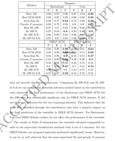
4. To evaluate whether the proposed unsupervised approach to RL can
out-perform recently proposed semi-supervised and unsupervised RL methods
and achieve comparable results to supervised classification methods such
ACCEPTED MANUSCRIPT
The proposed self-learning SVM-SGD ensemble method has been
imple-mented in Java with the Weka and Simmetrics Java libraries for SVM-SGD
classification and string similarity measures respectively. Five commonly used
similarity measures for RL have been used, namely Jaro (J), Smith-Waterman
(SW), Q-Gram (Q), Jaro-Winkler (JW) and Levenshtein edit distance (L).
How-ever, any other similarity measures could be applied.
The experiments were conducted with four datasets commonly used for
eval-uating RL methods: Restaurant1, Cora1, ACM-DBLP2 and DBLP-Scholar2.
The Restaurant dataset contains 864 restaurant records (372,816 record pairs
with 112 pairs of matching records), each with five fields, including name,
ad-dress, city, phone and type. The Cora dataset is a collection of 1,295 (837,865
record pairs with 17,184 pairs of matching records) citations to computer
sci-ence papers. Each citation is represented by 4 fields (author, title, venue, year).
The ACM-DBLP and DBLP-Scholar are a bibliographic datasets of Computer
Science bibliography records represented by four attributes. The total number
of entity pairs (cross product) is 6,001,104 and 168,181,505 for ACM-DBLP and
DBLP-Scholar respectively.
5.1. Automatic Seed Selection
We first evaluated whether the proposed technique for field weighting for seed
selection improves the performance of the self-learning algorithm. The algorithm
for automatic seed selection takes two parameters as input,mM andmU, which
specify the minimum numbers of match and non-match seeds that need to be
selected in the first phase of the seed selection process. We usedmU = 1% of
the total number of similarity vectors and a smaller value ofmM = 0.01% due
to the imbalanced distribution of match and non-match examples. Commonly
in RL the number of matching pairs of records is significantly smaller than the
number of non-matches. Therefore, the value ofmM needs to be smaller. If we
1https://www.cs.utexas.edu/users/ml/riddle/data.html
2http://dbs.uni-leipzig.de/en/research/projects/object_matching/fever/
ACCEPTED MANUSCRIPT
set it too high we could get a large number of false positive seeds. Since the
number of non-matches is much larger than the one of matches we can allow for
mU to be much higher to provide a bigger set of seeds.
We compared the precision and recall of the seeds selected in two phases.
Phase I is where the seeds are selected using unweighed Manhattan distance.
Phase II is where the seeds selected in Phase 1 are used to calculate the weights
of fields and then the final seeds are selected using the weighted Manhattan
distance. The results are presented in Tables 4-7. Due to the large initial pool
of the similarity measure schemes generated in Step 2, we only compared the
results for the 10 most diverse sets of seeds selected in Step 4. The second
column in each of the tables indicates which similarity measure scheme was
selected for generating the ensemble with each of the datasets.
Table 4: Precision and Recall of the seeds selected for the Restaurant dataset without (Phase I) and with (Phase II) field weighting
Phase I Phase II
Precision Recall Precision Recall
BC Sim. Scheme M NM M NM M NM M NM
1 J + J +J +J +J 0.91 1 0.13 0.01 0.86 1 0.45 0.02
2 J + J +J +J +Q 0.96 1 0.18 0.01 0.18 1 0.2 0.3
3 J + Q +J +J +J 0.95 1 0.16 0.01 0.93 1 0.13 0.04
4 Q + J +J +J +Q 0.95 1 0.36 0.01 1 1 0.73 0.9
5 Q + J +J +Q +J 0.98 1 0.36 0.1 1 1 0.73 0.89
6 Q + J +J +Q+Q 0.94 1 0.16 0.02 1 1 0.73 0.9
7 Q + Q+J +J +J 0.92 1 0.3 0.01 1 1 0.74 0.91
8 Q + Q +J +J +Q 0.97 1 0.1 0.02 1 1 0.73 0.9
9 Q + Q +J +Q +J 0.97 1 0.27 0.03 1 1 0.72 0.89
10 Q + Q +J +Q +Q 0.92 1 0.3 0.05 1 1 0.73 0.91
With the Restaurant dataset, in three out of ten cases (cases 1-3) better
precisions of the match seeds were obtained in Phase I. In the other cases better
results for match seeds were obtained in Phase II. For the non-match seed
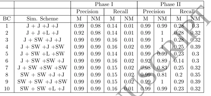
sig-nificantly better results were obtained in Phase II. For the Cora dataset, apart
from cases 6-8, better precision and recall of both match and non-match seeds
ACCEPTED MANUSCRIPT
Table 5: Precision and Recall of the seeds selected for the Cora dataset without (Phase I) and with (Phase II) field weighting
Phase I Phase II
Precision Recall Precision Recall
BC Sim. Scheme M NM M NM M NM M NM
1 J + J +J +J 0.99 0.98 0.14 0.01 0.99 0.99 0.28 0.3
2 J + J +L +J 0.92 0.98 0.14 0.01 0.99 1 0.28 0.32
3 J + SW +J +J 0.99 0.99 0.16 0.01 0.99 1 0.28 0.32
4 J + SW +J +SW 0.99 0.99 0.16 0.02 0.99 1 0.25 0.39
5 J + SW +L +SW 0.99 0.99 0.14 0.01 0.99 0.99 0.23 0.3
6 J + SW +SW +J 0.99 0.99 0.16 0.02 0.92 0.89 0.14 0.3
7 J + SW +SW +SW 0.99 0.99 0.15 0.02 0.98 0.83 0.25 0.32
8 SW + SW +J +J 0.99 0.99 0.15 0.02 0.99 0.81 0.2 0.35
9 SW + SW +J +SW 0.99 0.99 0.15 0.02 0.99 1 0.29 0.39
10 SW + SW +L +J 0.99 0.99 0.16 0.01 0.99 0.99 0.23 0.32
Table 6: Precision and Recall of the seeds selected for the DBLP-ACM dataset without (Phase I) and with (Phase II) field weighting
Phase I Phase II
Precision Recall Precision Recall
BC Sim. Scheme M NM M NM M NM M NM
1 J + J +J +J 0.73 0.99 0.1 0.63 0.73 0.99 0.1 0.63
2 J + L +J +J 0.72 1 0.09 0.73 0.67 0.98 0.27 0.9
3 J + SW +J +J 0.66 0.99 0.09 0.74 0.36 0.99 0.29 0.87
4 J + Q +J +J 0.75 0.99 0.11 0.79 0.9 0.99 0.43 0.9
5 L + Q +J +J 0.79 0.99 0.12 0.9 0.86 0.99 0.4 0.93
6 SW + J +J +J 0.86 0.99 0.4 0.9 0.91 0.99 0.35 0.93
7 SW + Q +J +J 0.84 0.99 0.4 0.93 0.86 0.99 0.42 0.93
8 Q + J +J +J 0.73 0.99 0.1 0.83 0.9 0.99 0.2 0.93
9 Q + SW +J +J 0.72 0.99 0.1 0.83 0.89 0.99 0.26 0.93
10 Q+Q+J+J 0.84 0.99 0.4 0.9 0.94 0.99 0.27 0.93
(M precision) and 6, 10 (M Recall) better match and non-match seeds were
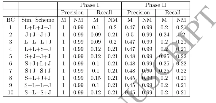
ob-tained in Phase II. For the DBLP-Scholar dataset the better results in term of
recall were obtained in Phase II for both matches and non-matches. However,
much better precision for matches was obtained in Phase I. It can be observed
from the results that in majority of the cases higher precision and higher recall,
ACCEPTED MANUSCRIPT
Table 7: Precision and Recall of the seeds selected for the DBLP-Scholar dataset without (Phase I) and with (Phase II) field weighting
Phase I Phase II
Precision Recall Precision Recall
BC Sim. Scheme M NM M NM M NM M NM
1 L+L+J+J 1 0.99 0.1 0.2 0.47 0.99 0.2 0.21
2 J+J+J+J 1 0.99 0.09 0.21 0.5 0.99 0.24 0.2
3 L+L+L+J 1 0.99 0.09 0.2 0.47 0.99 0.2 0.21
4 L+L+S+J 1 0.99 0.12 0.21 0.47 0.99 0.2 0.21
5 S+J+J+J 1 0.99 0.12 0.21 0.48 0.99 0.25 0.22
6 S+J+L+J 1 0.99 0.1 0.21 0.48 0.99 0.25 0.22
7 S+J+S+J 1 0.99 0.1 0.21 0.48 0.99 0.25 0.22
8 S+L+J+J 1 0.99 0.15 0.21 0.45 0.99 0.2 0.21
9 S+L+L+J 1 0.99 0.1 0.21 0.45 0.99 0.2 0.21
10 S+L+S+J 1 0.99 0.12 0.21 0.45 0.99 0.2 0.21
datasets apart from the DLBP-Scholar dataset. We presume that the low
pre-cision for DBLP-Scholar could be caused by the large number of missing values
in this dataset. Because of the missing values the algorithm was not able to
determine the weights correctly which caused a large number of false positive
seeds. This issue will be addressed in the future work.
In order to see how the quality of the seeds affects the self-learning process,
for each set of seeds from Tables 4-7 we evaluated the performance of the
self-learning model. Each of the diagrams in Figure 4 shows theF-measure obtained
by the self-learning models for each of the 4 datasets. For each of the datasets,
the self-learning process was performed with the similarity vectors generated
with each of the 10 selected similarity schemes. The self-learning process was
performed with field weighting (we refer to this method as SL-AW) and without
field weighting (we refer to this method as SL). Note that the self-learning
without field weighting is the same as the method proposed and evaluated in
[12]. It can be noted that for the Cora dataset the SL-AW performed better than
SL for each of the similarity schemes apart from cases 6-8, which is in line with
the results presented in Table 5. For the Restaurant dataset, the SL method
ACCEPTED MANUSCRIPT
row in Table 4 that for the same similarity measure scheme significantly better
precision of match seeds was obtained with the SL method. At the same time,
it can be noted that even though for similarity measure schemes 1 and 3 better
match seeds were selected with SL, the SL-AW method still performed better
in term of F-measure. This could be due to the fact that the precision and
recall of the non-match seeds were slightly better with the SL-AW in those
two cases. For the DBLP-ACM dataset the SL method performed equally or
slightly better than SL-AW in 4 cases (1, 3, 6 and 10). It can be observed from
the corresponding rows in Table 6 that for each of the four similarity measure
schemes SL obtained either better precision or recall of the match seeds. It can
be observed from Figure 4 that even though for the DBLP-Scholar dataset the
SL method had much higher precision that SL-AW, it performed better only in
four cases (4, 5, 8, 10). The reason for this could be the higher recall for the
matches obtained by SL-AW.
0 0.2 0.4 0.6 0.8 1
1 2 3 4 5 6 7 8 9 10 Restaurant SL SL-AW 0 0.2 0.4 0.6 0.8 1
1 2 3 4 5 6 7 8 9 10 Cora SL SL-AW 0 0.2 0.4 0.6 0.8 1
1 2 3 4 5 6 7 8 9 10 DBLP-ACM SL SL-AW 0 0.1 0.2 0.3 0.4 0.5 0.6 0.7
1 2 3 4 5 6 7 8 9 10 DBLP-SCHOLAR
SL SL-AW
ACCEPTED MANUSCRIPT
To further explore the relation between seeds and the final output of the
self-learning process we measured the correlation