VARIANCE HETEROGENEITY IN GENETIC MAPPING

VARIANCE HETEROGENEITY IN GENETIC MAPPING

Robert Wallace Corty

A dissertation submitted to the faculty of the University of North Carolina at Chapel Hill in partial fulfill- ment of the requirements for the degree of Doctor of Philosophy in the Curriculum of Bioinformatics and Computational Biology

Chapel Hill 2018

Approved by:

Fernando Pardo Manuel de Villena James Evans

Yun Li

Lisa Tarantino

© 2018

Robert Wallace Corty

ALL RIGHTS RESERVED

ABSTRACT

Robert Wallace Corty: Variance Heterogeneity in Genetic Mapping (Under the direction of William Valdar)

Genetic mapping is a process by which researchers seek to identify genetic factors that influence a trait of interest. Such efforts typically focus on those that either increase or decrease the trait of interest, and assume that the variance of the trait is constant across all individuals. I develop and apply statistical methods that challenge that assumption in two ways. First, I consider the situation where non-genetic factors influence trait variance, which I term “background variance heterogeneity”.

Though they are not of immediate interest in a genetic mapping study, they can be exploited to align observations’ weights with their precisions. Second, I consider the situation where genetic factors influence trait variance, which I term “foreground variance heterogeneity”. Such factors are of immediate interest because they represent novel discoveries that could be missed by standard analyses.

I consider both foreground and background variance heterogeneity as they relate to linkage disequilibrium mapping in exchangeable mapping populations. I report three novel genetic factors with strong evidence that they influence medically-important traits in the mouse model system.

Finally, I consider the background variance heterogeneity as it relates to association mapping in

non-exchangeable populations. I report a mathematical advance that makes possible the fitting

of a statistical model that accommodates background variance heterogeneity in non-exchangeable

populations.

Happy families are all alike;

every unhappy family is unhappy in its own way.

— Leo Tolstoy, opening line of Anna Karenina, on happiness-dependent variance heterogeneity

I’m convinced the tuxedo was invented by women. . . “Well, they’re all the same; we might as well dress them all the same.”

— Jerry Seinfeld,

on ignoring variation

ACKNOWLEDGEMENTS

I thank the Valdar lab for being a supportive and enriching venue in which to work and learn these past five years. I appreciate the efforts Will has made to create this lab environment by recruiting talented students such as Greg Keele, Paul Maurizio, Dan Oreper, Wes Crouse, Yanwei Cai, and Kathie Sun.

I thank the BCB program. They built it and we came. Tim Elston, Jonathan Cornett, and Cara Marlow were supportive in a thousand little ways that helped me stay focused on my academics.

I thank the MD-PhD program. The “big picture” guidance and support I’ve received from Gene Orringer, Toni Darville, Mohanish Deshmukh, Alison Regan, Carol Herion has kept me moving forward in a productive direction no matter how thick the morass of graduate school felt.

I thank my family. My mom, dad, and brother have been patient with me when I needed it and gave me a little kick sometimes when I needed that too.

I especially want to thank my grandparents. From childhood, my mom’s parents shared with me

a love of reading and writing. At every step in life, the value of these skills seems to compound. My

dad’s parents brought in another piece of the puzzle. With visits to the Franklin institute and a home

experimenter kit, they kindled my enthusiasm for science. I’m thrilled to be where I am and I am

deeply grateful to them for helping me get here.

TABLE OF CONTENTS

LIST OF TABLES . . . . ix

LIST OF FIGURES . . . . x

LIST OF ABBREVIATIONS . . . xiii

1 Introduction . . . . 1

1.1 Genetic Mapping . . . . 1

1.2 Variation and Variance . . . . 3

1.3 Sources of Variance . . . . 4

1.4 Variance Heterogeneity . . . . 8

1.5 QTL Mapping in the Presence of Variance Heterogeneity . . . 10

Linkage Disequilibrium Mapping in Exchangeable Populations 13 2 Mean-Variance QTL Mapping on a Background of Variance Heterogeneity . . . 14

2.1 Introduction. . . 14

2.2 Statistical Methods . . . 14

2.3 Data and Simulations . . . 23

2.4 Results . . . 27

2.5 Discussion . . . 38

2.6 Additional Information . . . 42

3 Mean-Variance QTL Mapping Identifies Novel QTL for Circadian Activity and Exploratory Behavior in Mice . . . 56

3.1 Introduction. . . 56

3.2 Statistical Methods . . . 56

3.3 Reanalysis of Kumar et al. Reveals a new mQTL for Circadian Wheel

Running Activity . . . 60

3.4 Reanalysis of Bailey et al. Identifies a new vQTL for Rearing Behavior . . . 63

3.5 Discussion . . . 67

3.6 Additional Information . . . 69

4 vqtl: An R package for Mean-Variance QTL Mapping . . . 77

4.1 Introduction. . . 77

4.2 Example data: Simulated F2 Intercross . . . 77

4.3 Scan the Genome . . . 78

4.4 Communicate Significant Findings . . . 84

4.5 Establish a Confidence Interval for the QTL . . . 85

4.6 Performance Benchmarks . . . 86

4.7 Conclusion . . . 88

4.8 Resources . . . 88

4.9 Phenotypes with Background Variance Heterogeneity . . . 89

Association Mapping 89 5 The Heteroscedastic Linear Mixed Model . . . 92

5.1 The Linear Mixed Model . . . 93

5.2 Compact Specification of the LMM . . . 94

5.3 Given h ² , the LMM problem reduces to the GLS problem . . . 95

5.4 Given M, the GLS problem reduces to the OLS problem . . . 95

5.5 M for the Homoscedastic LMM . . . 98

5.6 M for the Heteroscedastic LMM . . . 100

5.7 Simulation Studies . . . 103

5.8 Software . . . 110

6 Conclusion and Future Directions . . . 111

6.2 Outstanding Specific Aims. . . 112

6.3 Human Studies . . . 113

BIBLIOGRAPHY . . . 114

LIST OF TABLES

1.1 Sources of variance in measurements of a single organism. . . . 7

1.2 Sources of variance in measurements of multiple organisms. . . . 7

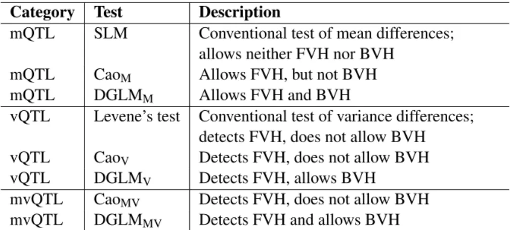
2.1 The eight tests that were evaluated in the simulation studies. . . 23

2.2 Positive rates of mQTL, vQTL, and mvQTL tests. . . 33

2.3 Positive rates of mQTL tests in extended scenarios. . . 50

2.4 Positive rates of vQTL tests in extended scenarios. . . 51

2.5 Positive rates of mvQTL tests in extended scenarios. . . 52

3.1 Genetic Variants in QTL interval for circadian wheel running activity . . . 64

3.2 The characteristics of the mice plotted in Figure 3.3 . . . 69

LIST OF FIGURES

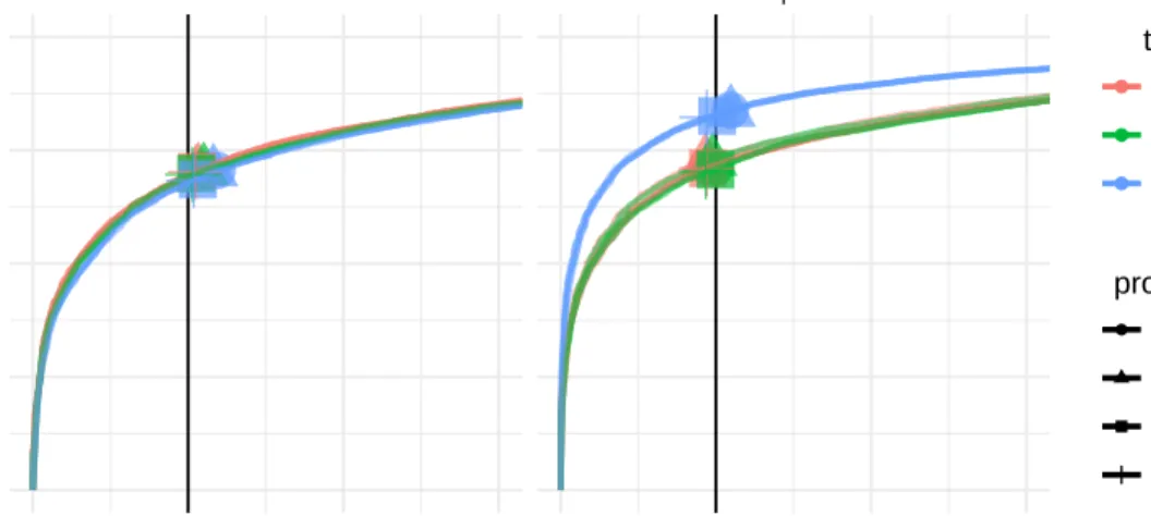
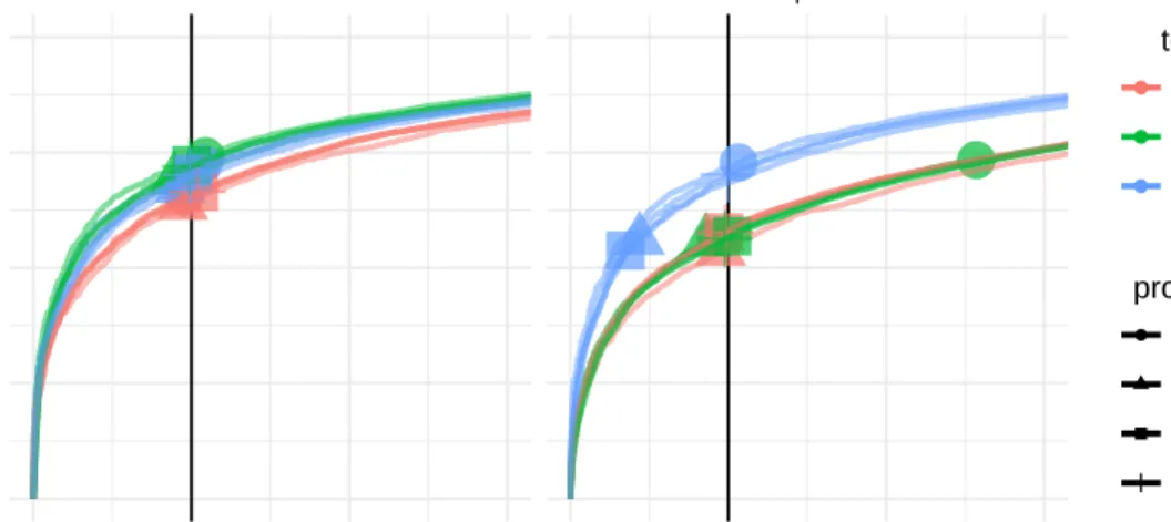
2.1 ROC curves for detection of mQTL in presence and absence of BVH. . . 28

2.2 ROC curves for detection of vQTL in presence and absence of BVH. . . 29

2.3 ROC curves for detection of mvQTL in presence and absence of BVH. . . 31

2.4 FWER-controlling association statistic at each genomic locus for body weight at three weeks. . . 34

2.5 Residuals from the standard linear model for body weight at three weeks, with sex and father as covariates, stratified by father. . . 36

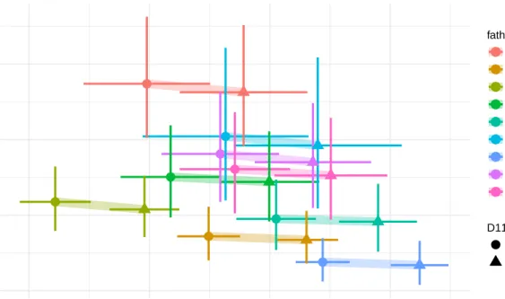
2.6 The predictive mean and standard deviation of mice in the mapping pop- ulation based on father and genotype at the top marker, D11MIT11 on chromosome 11. . . 37

2.7 ROC Curves for mQTL tests in the detection of mQTL. . . 44

2.8 ROC Curves for vQTL tests in the detection of vQTL. . . 45

2.9 ROC Curves for mvQTL tests in the detection of mvQTL. . . 46

2.10 The empirical false positive rate of each mQTL test-version for each nominal false positive rate, α, in [0, 0.1]. . . 47

2.11 The empirical false positive rate of each vQTL test-version for each nomi- nal false positive rate, α, in [0, 0.1]. . . 48

2.12 The empirical false positive rate of each mvQTL test-version for each nominal false positive rate, α, in [0, 0.1]. . . 49

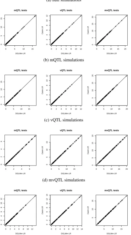
2.13 On simulated null loci, mQTL, vQTL, and mvQTL, Cao’s profile likeli- hood method had identical likelihood ratio to DGLM when DGLM does not use any variance covariates. . . 53

2.14 Genome scans conducted with the DGLM, without accounting for effects of sex and father on variance, shown by simulation to be identical to Cao’s tests (Figure 2.13, Table 2.3, Table 2.4, and Table 2.5). . . 54

2.15 Genome scans conducted with the DGLM, accounting for effects of sex and father on variance. . . 55

3.1 Genome scan for Kumar et al. circadian wheel running activity. . . 61

3.2 (a) Average wheel speed (revolutions/minute) of all mice. (b) Predicted

mean and variance of mice according to sex and allele at the QTL. . . 63

3.3 Double-plotted actograms illustrate the variation in wheel running activity

of male mice based on their genotype at rs30314218. . . 64 3.4 Genome scan for Bailey et al. rearing behavior. . . 66 3.5 (a) “Total Rearing Events”, transformed by the Box-Cox procedure, strat-

ified by sex and genotype at the top marker. (b) Predicted mean and

variance of mice according to sex and allele at the top marker. . . 66 3.6 Replicated scans from Kumar et al. (2013) . . . 69 3.7 Actograms, similar to Figure 3.3, including female mice. The mice de-

picted here are highlighted with larger circles in Figure 3.2a. . . 70 3.8 Page one of Mkrn1 alignment. Note that the amino acid at position 346 is

conserved across all species. See next page for species labels. . . 71 3.9 Page two of Mkrn1 alignment. . . 72 3.10 Replication of genome scans from original Bailey analysis. LOD curves

are visually identical to originally-published LOD curves, but thresholds,

estimated based on the described methods, are meaningfully higher. . . 73 3.11 DGLM-based reanalysis of all traits measured in Bailey et al., all trans-

formed by the rank-based inverse normal transform. . . 74 3.12 DGLM-based reanalysis of all traits measured in Bailey et al., all trans-

formed by the Box-Cox transform. Box-Cox exponents were 1, 1, 0, 0.75,

0, 0.25, respectively. . . 75 3.13 vQTL for TOTREAR phenotype on chromosome 2 is consistent across

various transforms. . . 76

4.1 LOD score of each test for each of the four simulated phenotypes. . . 80 4.2 FWER-corrected p-value of each test for each of the four simulated pheno-

types. . . 82 4.3 mean var plots show the estimated genotype effects at a locus with

mean effects on the horizontal axis and variance effects on the vertical axis. . . 84 4.4 Time taken to run scanonevar.perm on the data from Kumar et al.

(2013) which contains 244 individuals and 582 loci, varying the number

of permutations desired and the number of computer cores used. . . 86 4.5 Time taken to run 1000 permutation scans on 32 cores on simulated data

using scanonevar.perm, varying the number of individuals in the

mapping population and the number of markers in the genome. . . 87

4.6 LOD score of each test for each of the four simulated phenotypes with

4.7 Genomewide p-value of each test for each of the four simulated phenotypes

with background variance heterogeneity. . . 90

4.8 mean var plots show the estimated genotype effects at a locus, with mean effects on the horizontal axis and variance effects on the vertical axis. . . 91

5.1 Example quantile-quantile (QQ) plot. . . 105

5.2 QQ plots for simulations with 50 organisms in the mapping panel. . . 107

5.3 QQ plots for simulations with 100 organisms in the mapping panel. . . 108

5.4 QQ plots for simulations with 200 organisms in the mapping panel. . . 109

5.5 Receiver operating characteristics (ROC) curve for a GWAS with 100

organisms on a trait with h ² = 0.05. . . 110

LIST OF ABBREVIATIONS

DGLM double generalized linear model EMMA efficient mixed model analysis FPR false positive rate

FWER family-wise error rate GLS generalized least squares

ISAM inbred strain association mapping

LD linkage disequilibrium

LMM linear mixed model

LRT likelihood ratio test

ML maximum likelihood

mQTL mean-controlling quantitative trait locus

mvQTL mean or variance controlling quantitative trait locus

SLM standard linear model

QTL quantitative trait locus

vQTL variance-controlling quantitative trait locus

CHAPTER 1 Introduction

1.1 Genetic Mapping

Genetic mapping is a scientific endeavor that has elucidated the genetic underpinnings of hundreds of conditions relevant to human health and disease, both directly in humans (MacArthur et al., 2017) and in model organisms (Grubb et al., 2014), as well as many commercially-important traits in crops and livestock. There are, broadly speaking, three approaches to genetic mapping, which I will discuss below. They are united in their goal and the general process by which they seek to achieve it.

All approaches to genetic mapping involve the collection of phenotype and genotype information on a population of organisms and a statistical analysis to test for associations between the phenotype and each measured, polymorphic locus of the genome. This endeavor is motivated by the belief that the vast majority of the genome, say greater than 99%, does not have any appreciable effect on the phenotype, so a successful genetic mapping experiment allows researchers interested in the phenotype to focus their efforts on the small section of the genome that does have an effect. Thus, a successful genetic mapping effort results in a partition of the genome into a large part with no appreciable effect on the trait of interest, and a small part believed with a high degree of certainty to influence the phenotype.

The three general approaches to genetic mapping are: 1. linkage analysis, 2. linkage disequilib- rium mapping, and 3. association mapping. I’ll briefly review these approaches and some examples of how each has been productively applied.

Linkage Analysis is most useful for traits where one or a few genetic factors are expected to exert a

large effect (Elston and Stewart, 1971; Haseman and Elston, 1972). It is based on a large collection

of families with a few individuals per family, where each family must have at least one affected

and one unaffected individual and everyone has been genotyped across a sparse panel of markers.

Examples of successful applications of linkage analysis are Mendelian disease phenotypes like Duchenne muscular dystrophy, (Brown et al., 1985; Murray et al., 1982) cystic fibrosis (Tsui et al., 1985; Wainwright et al., 1985; White et al., 1985) and ataxia-telangiectasia (Gatti et al., 1988). In the last decade, as denser marker panels have become available and many of the high-prevalence, near-Mendelian traits have been mapped, linkage analysis has receded in prominence.

Linkage disequilibrium mapping involves an experimental population of organisms where the pattern of descent from a reference population can be inferred. For that reason, it is only possible in model organisms, livestock, and some crops — but never in humans. Strengths of this approach include the tight control of environmental exposures and the opportunity to deeply and invasively measure phenotypes. Two of the most classic designs, the F2 intercross and backcross, mimic the pedigrees of human linkage mapping, but rather than using many families with a few individuals per family, they create a single family with hundreds of siblings (Lynch and Walsh, 1998; Lander and Green, 1987; Lander and Botstein, 1989). Because these designs restrict the total genetic variation to only two parental haplotypes, rather than the vast number of haplotypes represented in a collection of human families, they are able to detect smaller effects and are not restricted to analyze mono- or oligo-genic traits in the way that linkage analysis is.

Modern efforts toward model organism LD mapping have made prominent use of more elab- orate breeding designs, most prominently multi-parental outbred populations (Ghazalpour et al., 2012; Svenson et al., 2012) and multi-parental genetic reference populations (The Complex Trait Consortium, 2004; MacKay et al., 2012; King et al., 2012) as well as in commercially-important crops (McMullen et al., 2009; Bandillo et al., 2013). These designs use a larger number of parental haplotypes and therefore explore a larger space of possible genetic effects than classic designs like F2’s and backcrosses. In this way, multi-parental populations designed for LD mapping strike a middle ground between classical designs and association analysis, which I discuss below.

Association mapping (GWAS) is based on a large population of individuals with no particular

genetic relationship. Because no breeding is required, it can be conducted in human populations. It is

most appropriate for traits where many genetic factors are thought to exert an effect, like body mass

index (Speliotes et al., 2010; Locke et al., 2015) and height (Allen et al., 2010; Wood et al., 2014)

and psychiatric conditions like schizophrenia (Ripke et al., 2014) and depression (of the PGC et al.,

2017). Each genetic locus is tested for association with the phenotype after a correction is made for global genetic similarity between individuals (Lippert et al., 2011; Zhou and Stephens, 2012).

Association mapping in model organisms uses a panel of inbred organisms with no particular genetic relationship to conduct a study similar to a human GWAS. This study design combines the strengths of model organism experiments (the tight control of environmental exposures and the ability to make invasive measurements) with the ability to observe replicates from each genome (Payseur and Place, 2007; Kang et al., 2008; Kirby et al., 2010). One important strength of a study design that allows multiple observations of the same genotype is that it allows for very precise measurement of the average phenotype that results from a given genotype because that genotype can be observed arbitrarily-many times. Additionally, it allows for direct quantification of environmental variance, which is confounded with genetic variance in any population without genetically-identical individuals (Falconer, 1965; Lynch and Walsh, 1998).

Across all these approaches to genetic mapping, the goal remains the same — to identify genetic loci where allelic variation correlates with phenotype variation.

1.2 Variation and Variance

We can say that we have observed “Variation” in some quantity when we have observed at least two different values for that quantity. Without phenotype variation, no analysis of any kind is possible, genetic or otherwise. Imagine a QTL mapping study where a tremendous amount of genotypic variation was measured, but, by chance, all individuals in the mapping population have the same phenotype value to measured precision. Realistically, the problem in such a study is that we did not measure the phenotype to sufficient precision — maybe the scale we used to measure mouse bodyweight was only accurate to the nearest pound, or maybe the phenotype is a molecular phenotype for which the state-of-the-art measurement procedure cannot differentiate between the highest and lowest values in our population. But more theoretically, given a set of observations without any variation, there can be no attempt to correlate it with variation in any other quantity, be they other phenotypes, environmental exposures, or genetic factors.

Analogously, for any genetic locus where all individuals in the mapping population have the

same allele, no genetic mapping study can hope to identify an association. This statement is quite

different from a mechanistic assessment that determines the gene products of this locus are irrelevant to the phenotype of interest; no such assessment can be made. Genetic mapping is fundamentally a statistical, rather than mechanistic process, simply testing for correlations between phenotype variation and allelic variation.

The above discussion considered variation as a binary quantity; it’s either present or absent. But there are a variety of measures that can be used to quantify variation. Some examples include the range, the interquartile range, the standard deviation, the mean absolute deviation, and the variance.

This dissertation deals almost exclusively with the variance because it has the salutary property that the sum of the variance attributable to each individual factor in a regression analysis is equal to the variance of the response (the phenotype in genetic applications). Put simply the variance of a sample of numbers is the sum of the squared differences between each number and the mean. For a large sample of numbers, this quantity accurately estimates the variance of the random process by which the numbers were generated.

At times, this dissertation also considers the standard deviation, which is simply the square root of the variance. The standard deviation has the property that it is on the same scale as the phenotype itself, and is therefore straightforwardly interpretable.

1.3 Sources of Variance

It is important to recognize all potential sources of variance in a population in which a genetic

mapping study will be conducted. Understanding genetic parameters such as broad sense and

narrow sense heritability, the percentage of variance explained by aggregate additive, dominance, and

epistatic effects yields valuable insights into the “genetic architecture” of the trait. Understanding

the effect of sex, bodyweight, and nuisance covariates such as housing, diet, and experimenter can

help scientists design more efficient experiments (Nettleton, 2006; Datta and Nettleton, 2014). I’ll

begin by reviewing sources of variance in measurements made on a single organism. As discussed

previously, in the absence of any genetic variation, there can be no prospect for genetic insight. I

continue with a review of sources of variance in measurements of multiple organisms, keeping in

mind that the single-organism sources of variance are still present.

1.3.1 Measurements on a Single Organism

There are surprisingly many sources of variance when multiple measurements are made, even on a single organism.

When multiple measurements of a given trait are made on a single individual at the same time, the only source of variance is technical variance (R¨onneg˚ard and Valdar, 2011). An example of this type of measurement is the collection of a single blood sample from a mouse, which is split it into three aliquots and the mRNA content of each aliquot is analyzed independently (Marioni et al., 2008).

When the a phenotype is measured on one individual at multiple times, temporal fluctuation is a potential source of variance. This temporal fluctuation comes in two “flavors”. First, the value of the phenotype of the individual may change over time. Second, the measurement device may change over time. Effects of this type are often called “batch effects”. An example of this type of measurement is the weighing of each experimental mouse each day of a multi-day experiment (Gray et al., 2015).

When the same organism is observed in multiple different “macro-environments”, that variation in macro-environment can contribute variance to the phenotype. The term “macro-environment” is used here to signify that the researcher has intentionally introduced an environmental effect. It is used in contrast to the “micro-environment”, which is discussed below. The same individual could be exposed to multiple different macro-environments at different times in its life, in which case temporal variation would potentially be in play, or samples of the organism can be extracted and treated with different environmental factors at a single time point.

When multiple, theoretically-identical structures are measured on a single individual at a single

time, “fluctuating asymmetry” is a potential source of variance (Palmer and Strobeck, 1986). An

example of this type of experiment is be measurement of the left and right kidney weight of mice

(Leamy et al., 2000, 2002). There are valid criticisms to be made about many specific measurements

that are said to reflect fluctuating asymmetry. For example, in the case of the left and right kidney in

a mouse, some difference in size might be expected due to the right kidney being crowded by the

liver during development. But the general concept, that of assessing the extent to which multiple

theoretically-identical phenotypes are expressed identically in a given organism, is an important

contribution to understanding the totality of sources of variance in a phenotype, for phenotypes where it is applicable.

A further source of variance in measurements of theoretically-identical structures from the same organism is developmental stochasticity. This term refers to the concept that micro-environmental perturbations during the developmental process can “fix” larger changes later in life, similar to a

“butterfly effect” of developmental biology.

1.3.2 Measurements on Multiple Organisms

When multiple organisms are observed, additional layers of variance are possible, depending on the genetics of the organisms (Table 1.2).

The experimental design that most limits the variance amongst multiple organisms is when all the organisms are genetically identical. In the observation of multiple genetically-identical organisms, developmental stochasticity, is a potential source of variation (Fraser and Schadt, 2010). This same source of variance can also be referred to as “micro-environmental variance” (Hill and Mulder, 2010).

This type of variance captures all the myriad, subtle exposures that each organism experiences, but which no researcher can hope to standardize. For example, the precise living temperature a mouse experiences depends slightly on where its cage is relative to the air vents, the amount of bedding depends on exactly how much the technician happened to grab when filling the cage, and uncountably many more such small effects could be imagined. Outside of experimental designs that make use of inbred organisms, it is impossible to directly estimate the contribution of micro-environmental variance to phenotype variance.

Consider a population of organisms that is not genetically identical in a global sense, but is genetically identical at one specific locus. A potential source of phenotype variance in such a population is interactions between the locus and factors in which the organisms do vary, such as other genetic loci and micro-environmental exposures. The fact that all the organisms have the same allele at the focal locus precludes any direct contribution from that locus to the phenotype variance.

But, the locus may interact with polymorphisms elsewhere in the genome to make a contribution

to the phenotype variance through GxG or may interact with micro-environmental factors to make

a contribution through GxE (Falconer and Mackay, 1995; Struchalin et al., 2010; R¨onneg˚ard and

sources of single or g anism v ariance measurement error or g anism fluctuation de vice fluctuation de v elopmental stochasticity macro-en vironment ef fects fluctuating asymmetry T able 1.1: Sources of v ariance that contrib ute to total phenotype v ariance in measurements of a single or g anism. Note that meas urement error is present in all measurements. Or g anismal fluctuation and de vice fluctuation ar e both the result of taking measurements at dif ferent times, b ut the y can be deconfounded with designs that cross indi viduals and de vices. sources of v ariance single or g anism v ariance de v elopmental stochasticity locus-by-G and locus-by-E mar ginal ef fects of all polymorphic loci one or g anism • genetically-identical or g anisms • • or g anisms with same allele at a locus • • • genetically-distinct or g anisms • • • • T able 1.2: Sources of v ariance that contrib ute to total phenotype v ariance in measurements of multiple or g anisms. The first column represents all the sources of v ariance that can be present in a measureme nt of a single or g anism (T able 1.1). Note the hierarchical nature of the sources of v ariance as we progress do wn the table from more-closely related indi viduals to less-closely related indi viduals; ne w sources of v ariance are added, b ut ne v er remo v ed.

Consider next a population of organisms where there are multiple alleles present at the focal locus — one could imagine the same population as the above paragraph but simply focus on a different locus. Here, all the same effects described above could be present, and additionally a marginal effect of the locus could contribute to phenotype variance. In fact, this is the reasoning that underlies the vast majority of QTL mapping efforts. Any genetic locus where researchers conclude with high statistical certainty that the proportion of phenotype variance explained by the locus is not zero constitutes a QTL (Broman and Sen, 2009; Broman, 2010).

Having considered thoroughly many possible sources of variance, I turn next to the concept that not all organisms are influenced by them to equal extent.

1.4 Variance Heterogeneity

Conceptually, any of the sources of variance described above could contribute more or less to any one measurement and any factor could determine how much a given source of variance contributes.

This situation is termed “variance heterogeneity”. The measurements could all end up with the same variance, and it’s simply partitioned differently according to sources. Or they could end up with different total variance.

Despite this reality, most genetics studies impose strong assumptions about the nature of pheno- type variation. They use statistical models that assume that each measurement has an equal quantity of variance from each source. To put a concrete example to that statement, the statistical analysis most commonly used in LD mapping of an F2 intercross or backcross assumes that the residual variance is constant across all individuals. In this study design, the “residual variance” is the sum of all within-individual sources of variance described above, the genomic variance arising from genetic factors other than the locus currently being tested (which I term the “focal locus”), locus-by-genome interactions, and locus-by-micro-environment interactions. So the assumption is equivalent to the belief that, across all organisms in the mapping population, that sum is equal.

Other study designs that are often analyzed with the assumption of homogeneous variance

include pedigree analysis to determine breeding values and heritability, inbred strain association

mapping, and human GWAS.

Despite the pervasiveness of these “constant variance” assumptions, there is ample evidence that these sources of variance do not affect each measurement equally. Rather this assumption arises out of analytic convenience. Statistical models that make use of the homogeneous variance assumption have been more straightforward to develop and tend to have faster performance than more complex models that allow for variance heterogeneity. This situation formed the central tension of my dissertation work. It was my belief that the analysis of many genetic study designs could be improved by using statistical models that recognize, and in some ways even capitalize on, variance heterogeneity.

1.4.1 Evidence of Variance Heterogeneity

Why might measurements from one organism have more variance than measurements from another organism? If one device is used for one organism and another device is used for another, heterogeneity of measurement error could result in heterogeneity of phenotype variance. Observations of this type have been made in the field of human blood pressure management (Labarthe et al., 1973;

Ataman et al., 1996; O’Brien, 2001).

As another example, genetic factors could influence phenotype variance by influencing sensitivity to variation in the micro-environment or influencing the extent of GxG or GxE variance. Family- based designs cannot disentangle these two sources of variance, but they can document their presence.

For example, genomic effects on phenotype variance have been documented in cattle (Visscher and Hill, 1992; Mulder et al., 2008; Fasoula, 2012), dairy cow (Clay et al., 1979), pigs (Ib´a˜nez-Escriche et al., 2008), chickens (Rowe et al., 2006), snails (Ros et al., 2004).

Other studies have documented a heterogeneity of phenotype variance across inbred strains, which can only be caused by differences in micro-environmental variation. Theses studies have documented this phenomenon in Drosophila melanogaster (Mackay and Lyman, 2005; Mackay, 2014), Arabidopsis thaliana (Hall et al., 2007), and crops (Walsh, 2017).

Early theoretical work focused on the notion that organisms with one allele at a locus might all have a similar phenotype, while organisms with the other allele might have very different phenotypes, despite tremendous variation in the rest of the genome in both groups and termed this phenomenon

“canalization” (Waddington, 1942, 1959). This work has been extended to include a population genetic

theory of how it could come about (Wagner et al., 1997; Gibson and Wagner, 2000; Meiklejohn

and Hartl, 2002). It has been related to the concept of “modularity” (Wagner et al., 2007), of

“developmental constraint” (Pavliˇcev and Cheverud, 2015). The original concept is now referred to as

“robustness” (Kitano, 2004; Felix and Barkoulas, 2015; Yadav et al., 2015; Fraser and Schadt, 2010) as well as “capacitance” (Pettersson and Carlborg, 2015; Queitsch et al., 2002). Usefully, the concept of robustness is divided into environmental robustness and genomic robustness (Fraser and Schadt, 2010), where the former refers to heterogeneity of locus-by-E variance and the latter to heterogeneity of locus-by-G variance.

1.5 QTL Mapping in the Presence of Variance Heterogeneity

Given the limited focus of the genetics community on variance heterogeneity, despite its seeming ubiquity, I sought to assess the ways in which it could damage QTL mapping efforts, through false positive or false negative results, and whether there were ways in which the presence of variance heterogeneity could actually strengthen genetic mapping efforts.

Quantitative trait locus (QTL) mapping in both model organisms and humans has traditionally focused on finding regions of the genome whose allelic variation influences the phenotypic mean.

In the past decade, a number of studies and proposed methods have broadened the scope of QTL

mapping to consider effects on the phenotypic variance (Par´e et al., 2010; R¨onneg˚ard and Valdar,

2011; Hulse and Cai, 2013). These studies and their findings have raised interesting questions and

possibilities about underlying biology, evolutionary trajectory, and potential utility in agriculture

(Wagner et al., 1997; Dworkin, 2005; Mulder et al., 2015). Nonetheless, consideration of variance

effects — whether as the target of inference or as a feature of the data to be accommodated — has

thus far remained outside of routine genetic analysis. This may be in part because QTL effects

on the variance are sometimes considered of esoteric secondary interest, intrinsically controversial

in their interpretation due to considerations of data scale (Sun et al., 2013; Shen and Ronnegard,

2013), or a priori too hard to detect (Visscher and Posthuma, 2010). But it is also likely to be in

part because familiar software and procedures are currently lacking, and because the advantages of

modeling heterogeneous variance, even when targeting QTL effects on the phenotypic mean, remain

under-appreciated and largely undemonstrated.

The predominant approach to QTL mapping in model organisms, the focus here, considers each genetic locus in turn, using a standard linear model (SLM) to regress the phenotypes of the mapping population on their genotypes or their inferred genotype probabilities (Lander and Botstein, 1989;

Haley and Knott, 1992). This SLM-based approach is primarily able to detect genomic regions containing a subset of genetic factors of interest — those that drive heterogeneity of phenotype mean.

Despite this limited scope, however, its use is widespread due to its ease of use, the straightforward interpretation of its detected QTL, its historical importance in the fields of agricultural and livestock genetics, and the fact that many genetic factors truly do influence the expected value of phenotypes.

Indeed, SLM-based interval mapping has yielded important insights on commercially- and medically- important traits across many organisms for many years.

The goal of QTL mapping, however, is much broader — to identify genetic factors that influence the phenotype in any way. For example, a genetic factor that influences the sensitivity of the phenotype to micro-environmental variation through a collection of what might be called a locus- by-E interactions is of interest whether the identity of the micro-environmental factors is known or not, but unless it also affects the mean it is undetectable by the SLM. Similarly, a genetic factor that influences the phenotype through many epistatic interactions (a collection of locus-by-G effects), but has an average effect near zero is unlikely to be detected by the SLM. Neither of these important goals, however, was the original motivation for seeking to detect genetic loci that influence phenotype variance. The original motivation was to lower the dimensionality of the search space for large locus-by-locus interactions (Par´e et al., 2010), by searching first for variants that influence the variance and then searching for interaction effects between those loci and the rest of the genome.

Such QTL that influence phenotype variance are often termed “vQTL”. The goal of detecting vQTL and other more exotic types of QTL effects motivated the development and application of statistical tests that can detect genetic effects on other aspects of the phenotypic distribution, most notably the phenotype variance.

A number of statistical models and methods have been developed or adapted to identify associ-

ations between genotype and phenotypic variance. These include: Levene’s test (Struchalin et al.,

2010), the Fligner-Killeen test (Fraser and Schadt, 2010), Bartlett’s test (Freund et al., 2013), the

double generalized linear model (DGLM) and similar (R¨onneg˚ard and Valdar, 2011; Cao et al., 2014),

and a host of two-step procedures that involve computing measure of variance for each individual and

testing that quantity for relation to the tested locus (Brown et al., 2014; Ayroles et al., 2015; Forsberg et al., 2015). Tests have also been developed to detect genotype associations with arbitrary functions of the phenotype, for example higher moments. These include a variant of the Komolgorov-Smirnov test (Aschard et al., 2013) and a semi-parametric exponential tilt model (Hong et al., 2016). The additional flexibility of these latter models makes them promising — a genetic factor that influences, e.g., the kurtosis of a phenotype should be of interest — but at present neither can accommodate covariates and the flexibility that affords them the ability to detect higher order effects brings with it a decreased power to detect mean and variance effects.

Efforts to identify vQTL have gathered steam in recent years. A few dozen vQTL have been reported, spanning Arabidopsis thaliana (Jimenez-Gomez et al., 2011; Shen et al., 2012; Forsberg et al., 2014), flowers (Lee et al., 2014), dairy cows (Fikse et al., 2012), Drosophila melanogaster (Ayroles et al., 2015; Huang et al., 2015), layer chickens (Wolc et al., 2012), maize (Ordas et al., 2008), mouse (Gray et al., 2015), and yeast (Nelson et al., 2013; Ziv et al., 2017; Forsberg et al., 2017). In at least two cases, researchers have identified vQTL and then gone on to identify specific interactions that caused the appearance of that vQTL (Huang et al., 2015; Brown, 2017), one of the original stated goals of vQTL analysis.

The existence of a vQTL, or indeed any factor affecting the variance has implications regarding statistical genetic analyses, both those targeting variance effects and those targeted mean-affecting QTL (hereafter, “mQTL”), and these implications have been relatively unexamined.

In particular, if a genetic (or other) factor influences phenotype variance then it follows that examination and testing of any other QTL effect — for example, that of a QTL elsewhere in the genome — must occur against a backdrop of systematically heterogeneous residual variance. The presence of this “background variance heterogeneity” (BVH) when testing for a (foreground) effect simultaneously presents analytic challenges and opportunities, not only for mapping vQTL but also the validity of studies detecting mQTL.

The impact of BVH on mapping mQTL can be thought of as a disruption of the natural observa-

tion weights: The SLM assumes the phenotype of every individual is subject to equal noise variance

and therefore equal weight; but if it is known that some individuals’ phenotypes are inherently less

noisy — due to BVH induced by either a vQTL or other factors such as sex, housing, strain or

for mQTL detection. Conversely, giving equal weight to subgroups of the data that are inherently noisier than average has the potential to leave outliers with overmuch influence on the regression, increasing the potential for false positive mQTL detections A case in point is when an mQTL also has variance effects: here the effects on the variance are a type of proximal BVH, and modeling them explicitly improves ability to detect effects on the mean, as in chapter 3. Knowledge and appropriate modeling of variance heterogeneity therefore has important implications for making mean-controlling QTL studies sensitive, robust and reproducible.

The impact of BVH on detection of foreground vQTL is more subtle. Parametric methods to identify vQTL typically pit heterogeneous variance alternative models against a homoskedastic, normally distributed null. However, under BVH the null model is not homoskedastic — it is a scale mixture — and this risks the null being rejected too readily. BVH could therefore lead to an inflated vQTL false positive rate.

If BVH is disruptive to QTL mapping generally, it is potentially valuable to incorporate it into the QTL mapping model when its source is known, and to use robustifying techniques to protect against it when its source is unknown. Accommodating BVH of known source is most naturally achieved through modeling covariate effects on the variance, something that is straightforward with the DGLM of R¨onneg˚ard and Valdar (2011) but not currently with other proposed methods.

Protecting BVH when its source is unknown is less obvious, but since the threat manifests through

sensitivity to distributional assumptions, natural contenders include side-stepping such assumptions

via non-parametric approaches, e.g., permutation testing, or reshaping the distribution prior to

analysis through variable transformation. Both have been considered in the vQTL context, with

permutation used in Hulse and Cai (2013) and Yang et al. (2012) and transformation in R¨onneg˚ard

and Valdar (2011), Yang et al. (2012), Sun et al. (2013), and Shen and Carlborg (2013), but not

specifically for controlling vQTL false positives in the presence of BVH.

CHAPTER 2

Mean-Variance QTL Mapping on a Background of Variance Heterogeneity ¹

2.1 Introduction

Here we examine the effect of modeled and unmodeled BVH on power and false positive rate when mapping QTL affecting the mean, the variance or both. In doing so we:

1. Develop a robust, straightforward procedure and software based on the DGLM that can be used for routine mQTL and vQTL analysis;

2. Compare alternative proposed methods for mQTL and vQTL analysis;

3. Show how incorporating BVH can improve power for detecting mQTL and vQTL;

4. Show how sensitivity to model assumptions can be rescued by variable transformation and/or permutation.

5. Illustrate the effect of modeling BVH in existing dataset, an F2 cross from Leamy et al, and discover a new QTL for bodyweight.

2.2 Statistical Methods

This section reviews four approaches for modeling the effect of a single QTL on the phenotypic mean and/or variance: the standard linear model, Levene’s test, Cao’s tests, and our preferred procedure based on the DGLM. For each approach we describe a set of alternative procedures for evaluating significance (i.e., calculating p-values) that provide varying degrees of protection against the impact of BVH and distributional assumptions more generally. The following section, Data and Simulations, then describes a simulation study that assesses the approaches and p-value procedures, and a dataset to which they are applied genomewide.

1

2.2.1 Definitions

We start by defining three partially overlapping classes of QTL:

mQTL: a locus containing a genetic factor that causes heterogeneity of phenotype mean, vQTL: a locus containing a genetic factor that causes heterogeneity of phenotype variance, and mvQTL: a locus containing a genetic factor that causes heterogeneity of either phenotype mean,

variance, or both — a generalization that includes the other two classes.

In addition, since we restrict our attention to QTL mapping methods that test genetic association with a phenotype one locus at a time, we distinguish two sources of variance effects:

Foreground Variance Heterogeneity (FVH): effects on the variance that arise from the locus under consideration (the focal locus);

Background Variance Heterogeneity (BVH): effects on the variance that arise from outside of the focal locus, e.g., from another locus or an experimental covariate.

2.2.2 Procedures to evaluate the significance of a single test

In comparing different statistical approaches and their sensitivity to BVH, namely the effect of BVH on power and false positive rate (FPR), it is important to acknowledge that various measures could be taken to make significance testing procedures more robust to model misspecification in general and to BVH specifically. The significance testing methods considered here are frequentist, involving the calculation of a test statistic T on the observed data followed by an estimation of statistical significance based on a conception of T ’s distribution under the null. However, BVH constitutes a departure of distributional assumptions, and in any rigorous applied statistical analysis when departures are expected it would be typical to consider protective measures such as, for example, transforming the response to make asymptotic assumptions more reasonable, or the use of computationally intensive procedures, such as those based on bootstrapping or permutation, to evaluate significance empirically.

Nominal significance (i.e., the p-value for a single hypothesis test) is evaluated using four distinct

procedures. The first two rely on asymptotics:

1. Standard: The test statistic T is computed on the observed data and compared with its asymptotic distribution under the null.

2. Rank-based inverse normal transform (RINT): As for standard, except observed phenotypes {y _i } ⁿ _i=1 are first transformed to strict normality using the function RINT(y _i ) = Φ ⁻¹ [(rank(y _i )−

3 / 8 )/(n + ¹ / 4 )], where Φ is the normal c.d.f. and rank(y _i ) is gives the rank (from 1, . . . , n) (Beasley et al., 2009).

The second two determine significance empirically based on randomization: the test statistic T is recomputed as T ^(r) under randomizations of the data r = 1, . . . , R, and the resulting set of statistics {T ^(r) } ^R _r=1 is used as the empirical distribution of T under the randomized null. Two alternative randomizations are considered:

3. Residperm: we generate a pseudo-null response {y _i ^(r) } ⁿ _i=1 based on permuting the residuals of the fitted null model, (Freedman and Lane, 1983; Good, 2013), a process recently applied in the field of QTL mapping by Cao et al. (2014).

4. Locusperm: we leave the response intact, instead permuting the rows of the design matrix (or matrices) that differentiate(s) the null from alternative model.

2.2.3 Procedure to evaluate genomewide significance

In the context of a genome scan, where many hypotheses are tested, we aim to control the genomewide FPR, namely the family-wise error rate (FWER), the probability of making at least one false positive finding across the whole genome. This is done following the general approach of Churchill and Doerge (1994), which is closely related to the locusperm procedure described above, and which we refer to as genomeperm. Briefly, we perform an initial genome scan, recording test statistics {T _l } ^L _l=1 for all L loci. Then for each randomization r = 1, . . . , R, and for only the parts of the model that distinguish the null from the alternative model, the genomes are permuted among the individuals; the scan is then repeated to yield simulated null test statistics {T _l ^(r) } ^L _l=1 of which the maximum, T max ^(r) , is recorded. The collection of {T max ^(r) } ^R _r=1 from all R such permutations is then used to fit a generalized extreme value distribution (GEV) (Dudbridge and Koeleman, 2004), and the

L

2.2.4 Standard linear model (SLM) for detecting mQTL

The standard model of quantitative trait mapping uses a linear regression based on the approxima- tion of Haley and Knott (1992) and Mart´ınez and Curnow (1992) to interval mapping of Lander and Botstein (1989). The effect of a given QTL on quantitative phenotype y i of individual i = 1, . . . , n is modeled as

y _i ∼ N(m _i , σ ² ) (2.1)

where σ ² is the residual variance and m i is a linear predictor for the mean, defined, in what we term the “full model”, as

Full model: m _i = µ + x ^T _i β + q ^T _i α , (2.2) where µ is the intercept, x _i is a vector of covariates with effects β, and q _i is a vector encoding the genetic state at the putative mQTL with corresponding mQTL effects α. In the case considered here of biallelic loci arising from a cross of two founders, A and B, the genetic state vector q i = (a i , d i ) ^T is defined as follows: when genotype is known, for genotypes (AA, AB, BB), the additive dosage is a i = (0, 1, 2) and the dominance predictor is d i = (0, 1, 0); when genotype is available only as estimated probabilities p(AA), p(AB) and p(BB), following (Haley and Knott, 1992; Mart´ınez and Curnow, 1992), we use the corresponding expectations, a i = 2p(AA) + p(AB) and d _i = p(AB).

The test statistic for an mQTL is based on comparing the fit of the full model, acting as an alternative model, with that of a null that omits the locus effect, namely,

Null model: m i = µ + x ^T _i β . (2.3)

Since the regression in each case provides a maximum likelihood fit, the test statistic used here is

likelihood ratio (LR) statistic, T = 2(` <sub>1</sub> − ` ₀ ), where ` <sub>1</sub> and ` ₀ are the log-likelihoods under the

alternative and the null respectively. For the biallelic model, the asymptotic test is the likelihood

ratio test (LRT) whereby under the null, T ∼ χ ² ₂ . (Note: Alternative evaluation using the F-test is in

general more precise but for our purposes provides equivalent results.)

The residperm approach to empirical significance evaluation of T proceeds as follows. We first fit the null model (Equation 2.3) to obtain predicted values m b i = x ^T _i β and estimated residuals ˆ ε b i such that y i = m b i + ε b i . Then, for each randomization r = 1, . . . , R, we generate pseudo-null phenotypes {y ^(r) _i } ⁿ _i=1 as

y _i ^(r) = m b i + b ε _π

_(i) ,

where if π _r is a vector containing a random permutation of the indices i = 1, . . . , n, then π _r (i) is its ith element, mapping index i to its rth permuted version. The null and alternative models are then fitted to {y ^(r) _i } ⁿ _i=1 to yield ` <sup>(r)</sup> <sub>1</sub> and ` ^(r) ₀ , and hence T ^(r) .

In the locusperm approach to empirical significance, the response is unchanged but permutations are applied to the locus genotypes. For each randomization r, the full model m i is

Permuted full model: m _i = µ + x ^T _i β + q ^T _π

r

(i) α (2.4)

where π r (i) is as defined for residperm above. This full model fit yields ` <sup>(r)</sup> <sub>1</sub> , and then T <sup>(r)</sup> = 2(` ^(r) ₁ − ` <sub>0</sub> ). Note that ` ^(r) ₀ need not be recomputed after randomization because because only the rows of the design matrices that are unique to the alternative model are permuted and thus ` <sup>(r)</sup> <sub>0</sub> = ` ₀ . Genomeperm applies locusperm genomewide: specifically, in each randomization r = 1, . . . , R, the same permutation, π r , is applied to all L loci.

2.2.5 Levene’s Test (LV) for detecting vQTL

Levene’s test is a procedure for differences in variance between groups that can be used to detect vQTL. Suppose individuals are in G mutually exclusive groups g = 1, . . . , G. Let g[i] denote the group to which individual i belongs, denote gth group size as n g = P n

i=1 I _{g[i]=g} , and gth group mean as ¯ y _g = n ⁻¹ _g P n

i=1 y _i I _{g[i]=g} . Then denote the ith absolute deviation as z _i = |y _i − ¯ y _g[i] |, the group mean of these as ¯ z _g = n ⁻¹ _g P _n

i=1 z _i I _{g[i]=g} and overall mean ¯ z = n ⁻¹ P _n

i=1 z _i . Levene’s W statistic is then

W = P G

g=1 n _g (¯ z _g − ¯ z) ² (G − 1)

" P n

i=1 (z _i − ¯ z _g[i] ) ² (n − G)

# −1

, (2.5)

which under the null model of no variance effect follows the F distribution as W ∼ F (N − G, G − 1)

test (Brown and Forsythe, 1973), and replacing all instances of z with y in Equation 2.5 gives the ANOVA F statistic.

Levene’s test does not lend itself naturally to the residperm approach because it does not explicitly involve a null model to split the data into hat values and residuals. We therefore use the null model from the SLM (Equation 2.3) to approximate the residperm procedure with Levene’s test.

To execute the locusperm procedure, for each randomization r, the group labels are permuted among the individuals, which is equivalent to replacing all instances of g[i] above with g[π r (i)], with π _r (i) defined as above. A corresponding genomewide procedure, although not performed here, would ensure that each randomization r applies the same permutation π _r across all loci.

2.2.6 Cao’s Tests

Cao et al. (2014) elaborates the SLM to have a variance parameter that differs by genotype, i.e.,

y i ∼ N(m _i , σ ² _i ), (2.6)

where m i is the linear predictor, σ ² _i is the variance of the ith individual. These are defined in what we term the “full model” as

Full model:



 



 



m _i = µ + x ^T _i β + q ^T _i α σ _i ² = φ _g[i]

, (2.7)

where g[i] indexes the genotype group to which i belongs, and {φ g } ^G _g=1 are the variances of the g = 1, . . . , G genotype groups. Thus an individual’s variance is entirely dictated by its genotype, and that genotype must be categorically known (or otherwise assigned). Cao et al. (2014) fits this model using a two-step, profile likelihood method, which in our applications we observe to be indistinguishable from full maximum likelihood (Figure 2.13).

Cao et al. (2014) describes tests for mQTL, vQTL and mvQTL based on comparing a full

model against three different null models; we detail these tests below in our notation, denoting them

respectively Cao _M , Cao _V , and Cao _MV .

2.2.6.1 Cao M test for detection of mQTL

The Cao _M test involves an LRT between Cao’s full model and Cao’s no-mQTL model:

Cao’s no-mQTL model:



 



 



m i = µ + x ^T _i β σ _i ² = φ _g[i]

, (2.8)

To execute the residperm procedure for Cao _M , pseudo-null phenotypes are generated using m b i and ε b i

from Cao’s no-mQTL model (Equation 2.8). The locusperm procedure respecifies the full model (Equation 2.7), leaving the variance model unchanged and specifying the mean predictor as m i = µ + x ^T _i β + q ^T _π

r

(i) α. The genomeperm procedure similarly applies the locusperm procedure genomewide, ensuring each randomization r applies the same permutation π r to the mean specification across all loci.

2.2.6.2 Cao _V for detection of vQTL

The Cao V test involves an LRT between Cao’s full model and Cao’s no-vQTL model:

Cao’s no-vQTL model:



 



 



m _i = µ + x ^T _i β + q ^T _i α σ ² _i = σ ²

, (2.9)

where the unsubscripted σ ² is a single, overall residual variance. This null model is identical to the alternative model in the SLM (Equation 2.2).

To execute the residperm procedure for Cao _V , pseudo-null phenotypes are generating using m b _i

and ε b i from Cao’s no-mQTL model (Equation 2.9). The locusperm procedure respecifies the full

model (Equation 2.7), leaving the mean sub-model unchanged and specifying the variance predictor

as σ _i ² = φ _g[π(i)] . The genomeperm procedure applies the locusperm procedure genomewide, ensuring

each randomization r applies the same permutation π r to the variance specification across all loci.

2.2.6.3 Cao MV for detection of generalized mvQTL

The Cao _MV test involves an LRT between Cao’s full model and Cao’s no-QTL model:

Cao’s no-QTL model:



 



 



m i = µ + x ^T _i β σ ² _i = σ ²

. (2.10)

This null model is identical to the null model in the SLM (Equation 2.3).

To execute the residperm procedure for Cao _MV , pseudo-null phenotypes are generated using m b _i and b ε _i from Cao’s no-QTL model (Equation 2.10). The locusperm procedure specifies the mean predictor as m i = µ + x ^T _i β + q _π(i) and the variance predictor as σ _g[i] ² = φ _[π(i)] . The genomeperm procedure applies the locusperm procedure genomewide, ensuring each randomization r applies the same permutation π r to the mean and variance specifications across all loci.

2.2.7 Double Generalized Linear Model (DGLM)

The DGLM models the phenotype y i via two linear predictors as

y _i ∼ N(m _i , σ _i ² ) , where σ _i ² = σ ² × exp(v _i )

where m i predicts the phenotype mean and v i predicts the extent to which the baseline residual variance σ ² is increased in individual i. In what we term the “DGLM full model”, these are specified as

Full model:



 



 



m i = µ + x ^T _i β + q ^T _i α v _i = z ^T _i γ + q ^T _i θ

, (2.11)

where µ is the intercept, z i is a vector of covariates (which may be identical to x i ), γ is a vector of covariate effects on v _i , and θ is a vector of locus effects on v _i .

As with Cao’s full model, the DGLM full model can be compared, in a likelihood ratio test,

with various null models to test for mQTL, vQTL (R¨onneg˚ard and Valdar, 2011), or mvQTL. A full

maximum likelihood fitting procedure for the DGLM was provided by Smyth (1989).

2.2.7.1 DGLM M for detecting mQTL:

For detecting mQTL, we use an LRT of the DGLM full model in Equation 3.1 against the no-mQTL model:

No-mQTL model:



 



 



m _i = µ + x ^T _i β v _i = z ^T _i γ + q ^T _i θ

, (2.12)

where the LR statistic has asymptotic distribution T ∼ χ ² ₂ .

To execute the residperm procedure for DGLM _M , pseudo-null phenotypes are generated using m b i and b ε i from the Equation 2.12. The locusperm procedure respecifies the mean predictor as m i = µ + x ^T _i β + q ^T _π(i) α and does not modify the variance predictor. The genomeperm procedure similarly applies the locusperm procedure genomewide, ensuring each randomization r applies the same permutation π r to the mean specification across all loci.

2.2.7.2 DGLM _V for detecting vQTL:

For detecting vQTL, we use an LRT of the DGLM full model in Equation 3.1 against the no-vQTL model:

No-vQTL model:



 



 



m i = µ + x ^T _i β + q ^T _i α v _i = z ^T _i γ

, (2.13)

where the LR statistic has asymptotic distribution T ∼ χ ² ₂ .

To execute the residperm procedure for DGLM V , pseudo-null phenotypes are generated using m b i

and ε b i from the Equation 2.13. The locusperm procedure does not modify the variance predictor and

respecifies the mean predictor as v i = z ^T _i γ + q ^T _π(i) θ. The genomeperm procedure similarly applies

the locusperm procedure genomewide, ensuring each randomization r applies the same permutation

π _r to the variance specification across all loci.

Category Test Description

mQTL SLM Conventional test of mean differences;

allows neither FVH nor BVH

mQTL Cao _M Allows FVH, but not BVH

mQTL DGLM M Allows FVH and BVH

vQTL Levene’s test Conventional test of variance differences;

detects FVH, does not allow BVH vQTL Cao _V Detects FVH, does not allow BVH

vQTL DGLM V Detects FVH, allows BVH

mvQTL Cao _MV Detects FVH, does not allow BVH mvQTL DGLM MV Detects FVH and allows BVH

Table 2.1: The eight tests that were evaluated in the simulation studies. FVH: foreground variance heterogeneity. BVH: background variance heterogeneity.

2.2.7.3 DGLM MV for detecting mvQTL:

For detecting mvQTL, we use an LRT of the DGLM full model in Equation 3.1 against the no-QTL model:

No-QTL model:



 



 



m _i = µ + x ^T _i β v i = z ^T _i γ

, (2.14)

where the LR statistic has asymptotic distribution T ∼ χ ² ₄ .

To execute the residperm procedure for DGLM _MV , pseudo-null phenotypes are generated using m b i and b ε i from the Equation 2.14. The locusperm procedure respecifies the mean predictor as m i = µ + x ^T _i β + q ^T _π(i) α and the variance predictor as v i = z ^T _i γ + q ^T _π(i) θ. The genomeperm procedure similarly applies the locusperm procedure genomewide, ensuring each randomization r applies the same permutation π r to the mean and variance specifications across all loci.

2.3 Data and Simulations

Simulation was used to assess the ability of the eight tests described above to distinguish each

of the three types of QTL — pure mQTL, pure vQTL, and mixed mvQTL — from a null locus in

the presence and absence of background variance heterogeneity (BVH). Tests are distinguished by

their ability to accommodate and target foreground variance heterogeneity (FVH) and background

variance heterogeneity (Table 2.1).

In each simulation, n = 300 observations were simulated as

y i ∼ N(q ^T _i α, exp(z ^T _i γ + q ^T _i θ))

where y _i is the phenotype of individual i, q _i is the genotype, and z _i is the indicator vector for the factor that drives BVH in scenarios where it is present. In each simulation, each row of q (each q i ) is drawn randomly from [-1, 0, 1] with probability (0.25, 0.5, 0.25) mimicking an F2 intercross. Across all simulations, Z is fixed to be an indicator matrix mapping the first 60 observations to group 1, the next 60 to group 2, ... and the last 60 to group 5.

Values of α, θ, and γ differentiate the eight simulation scenarios as described below.

2.3.1 Scenarios

Simulations varied in two dimensions: locus effect (four options) and BVH (two options) for a total of eight simulation scenarios. Each of the eight scenarios was examined in S = 10, 000 simula- tion trials. Locus effect sizes were chosen such that all QTL were detectable with approximately 70% power at a 5% false positive rate for traditional tests in the absence of BVH. Comprehensive details on the simulation setup are described in Supplementary Materials.

The four options for a simulated locus effect were as follows:

1. null locus: The locus has no effect on phenotype.

2. pure mQTL: The locus has an additive effect on the phenotype mean that explains 5% of the total variance.

3. pure vQTL: The locus has an additive effect on the log standard deviation that is detectable with approximately 70% power at a 5% false positive rate for traditional tests in the absence of BVH.

4. mixed mvQTL: The locus has both an additive mean effect that explains 3.25% of phenotype variance and an additive variance effect that is approximately equally detectable.

The two options for simulated BVH were as follows:

1. absent: Nothing, except for possibly the locus (if a vQTL or mvQTL), influences the residual variance. (γ = [0, 0, 0, 0, 0])

2. present: γ = [−0.4, −0.2, 0, 0.2, 0.4], resulting in group-wise standard deviations in the null locus and mQTL scenarios of approximately [0.67, 0.82, 1, 1.22, 1.49]. In the vQTL and mvQTL scenarios, these BVH effects combine additively with the locus effects on the log standard deviation scale, yielding 15 distinct standard deviations. These effect sizes generate a spectrum of standard deviations across groups that are consistent with those observed in the real data reanalysis that follows.

2.3.2 Tests and Significance

In each scenario, eleven tests were applied, and four procedures were used to assess the statistical significance of each test, for a total of 32 test-procedures.

The eleven tests comprise four tests for detecting mQTL: LM, Cao M , and DGLM M with and without modeling the variance covariate; four for detecting vQTL: Levene’s test, Cao V , DGLM V with and without modeling the variance covariate; and three for detecting mvQTL: Cao MV and DGLM MV

with and without modeling the variance covariate, as described in Methods.

The eleven tests, however, contain some redundancy, and so in the main text we report results from only eight. Specifically, for a given type of QTL, the DGLM model that omits variance covariates is equivalent to the corresponding Cao’s test, and, barring computational errors in fitting, should give equivalent results (as was observed); results from these DGLM models are therefore omitted from the main text, but for completeness are reported in the supplement.

The four procedures for evaluating the statistical significance were: standard, RINT, residperm, and locusperm, as described in the Methods.

2.3.3 Evaluation of tests and procedures

Tests and procedures for assessing statistical significance were evaluated based on their receiver operating characteristics (ROC) and their ability to accurately control the FPR to the nominal level.

ROC curves display the ability of a test to discriminate between two conditions by plotting FPR

against power for all possible cutoffs.