Pseudo Goodwin cycles in a Minsky model

1 Pseudo-Goodwin cycles in a Minsky model

E. Stockhammer* and J. Michell**

Version 6.0, Jan 2016

Abstract. Goodwin cycles result from the dynamic interaction between a profit-led demand regime and a reserve army effect in income distribution. The paper proposes the concept of a pseudo-Goodwin cycle. We define this as a counter-clockwise movement in output and wage share space which is not generated by the usual Goodwin mechanism. In particular, it does not depend on a profit-led demand regime. As a demonstration, a simple Minsky model is extended by adding a reserve army distribution mechanism such that the wage share responds positively to output. In the extended Minsky model, cycles are generated purely through the interaction between financial fragility and demand. In a first step we assume no feedback from income distribution to demand. We demonstrate that the model generates a pseudo-Goodwin cycle in output-wage share space. In a second step, we show that the result continues to hold even if a wage-led demand regime is

introduced, although this can introduce instability. Our models demonstrate that the existence of a counter-clockwise movement of output and the wage share cannot be regarded as proof of the existence of a Goodwin cycle and a profit-led demand regime.

* Engelbert Stockhammer, Kingston University, Penrhyn Road, KT1 2EE Surrey, UK Email: [email protected]

Phone: +44 208 417 7774

** Jo Michell, University of the West of England, Coldharbour Ln, Bristol BS16 1QY

Acknowledgements. The authors are grateful to Johannes Buchner, Sebastien Charles, Paulo dos Santos, Giorgos Galanis, Rob Jump, Javier Lopez, Nina Kaltenbrunner, Marc Lavoie, Maria Nikolaidi, Hiroshi Nishi and Peter Skott for comments and two anonymous referees. The usual disclaimers apply.

Keywords: business cycles, Goodwin cycle, Minsky cycle, financial fragility, distribution cycles, Post Keynesian economics

2 Pseudo-Goodwin cycles in a Minsky model

Introduction

The question of how aggregate demand and income distribution interact to generate business cycles continues to generate considerable debate in the heterodox economics literature. One influential view is derived from Goodwin’s (1967) model, in which cycles are generated by the interaction between accumulation, which is savings-driven, and a reserve army distribution function. Since workers are assumed not to save, the Goodwin cycle posits that an increase in the wage share of output will have a negative effect on accumulation because a reduced profit share causes a fall in investment. Goodwin also assumes that the wage share will rise at higher levels of output because the bargaining power of labour increases as unemployment falls. The interaction of these two dynamic behavioural relationships produces a counter-clockwise cycle in output-wage share space. There is a related, on-going, debate about the nature of the demand regime in advanced economies. On one side are those who regard the demand regime as profit-led, in line with the assumptions of the Goodwin model (e.g. Taylor, 2012).1 On the other are those who argue that aggregate demand is wage-led (e.g. Stockhammer et al., 2009). These two strands of the literature intersect in studies which look for Goodwin-like patterns in empirical data and argue that such patterns provide support for the profit-led demand hypothesis: “A general finding is that ‘profit squeeze’ cycles exist for the US economy” (Barbosa-Filho and Taylor, 2006, p. 392; similar results are presented in Barbosa-Filho, 2015).

We take issue with this claim that the existence of a counter-clockwise movement in output-wage share space is proof of both a Goodwin cycle and a profit-led demand regime. Instead, we

demonstrate the existence of a pseudo-Goodwin cycle which we define as a counter-clockwise movement in output and wage share space that is not generated by the standard Goodwin mechanism. Specifically, it does not rely on a profit-led demand regime. Simply put, a pseudo-Goodwin cycle is something that looks like a pseudo-Goodwin cycle but isn’t.

To illustrate this we take a simple two equation predator-prey version of the Minsky model and add a reserve army distribution adjustment a la Marx and Goodwin. In Minsky’s model, the cycle results from an interaction between financial and real variables. In its simplest version, the theory states that demand and output growth give rise to higher debt ratios and financial fragility. This financial fragility has a negative effect on demand. As in the Goodwin model, these two dynamic behaviour relationships combine to produce cycles. In the Minsky model, these appear as clockwise

movements in output-fragility space.

3 To this simple formalisation of Minsky’s model, we add a reserve army effect such that the wage share rises with higher levels of output. The augmented Minsky model generates a pseudo-Goodwin cycle in output-wage share space. This is not a true Goodwin cycle because - by design - there is no mechanism by which distribution affects demand. Instead, the cycle is generated entirely by the interaction between demand and financial fragility. We demonstrate, further, that such pseudo-Goodwin cycles can still arise if we additionally assume a wage-led demand regime.

There have been some attempts at a synthesis of Goodwin and Minsky models (e.g. Keen 1995). These models specify feedbacks from both distribution and financial fragility to aggregate demand. Our paper, however, is asking a different question. We are interested, as a first step, in a model that has a Minsky cycle and a reserve army effect, but no feedback from distribution to demand. We know, by design, that the business cycle in this model will be driven by the finance-demand interaction. What the literature has not so far analysed is the question of what cyclical properties such a system will exhibit in output-distribution space. In other words, we are asking what a researcher looking for a Goodwin cycle would see, if he encountered a Minsky world with a reserve army distribution function. In a second step, we investigate Minsky models with both a reserve army effect and a wage-led demand regime.

The main purpose of the paper is one of theoretical clarification. The models presented are highly stylized. We use simple predator-prey models and, for the sake of clarity, we keep the number of parameters to a minimum. The baseline Goodwin and Minsky models on which we build generate stable cycles (closed orbits). We investigate the stability of the extended Minsky models, but our main concern is to establish the direction in which the cycle turns in output-wage share space. The paper is structured as follows. Section 2 presents a benchmark Goodwin model and discusses the related literature. Section 3 presents a simple Minsky model. Section 4 introduces a distribution function with a reserve army effect into the Minsky model and demonstrates the existence of pseudo-Goodwin cycles. Section 5 introduces a weak wage-led effect in the demand function. Section 6 presents a generalised version of the model that has a richer parameter structure and damping own-feedback effects. Section 7 concludes.

The Goodwin cycle

Goodwin (1967, 1972) presents a simple dynamic model of the cyclical interaction between employment and income distribution. The model is constructed on the basis of two key Marxian relationships. The first represents the reserve army assumption that as unemployment increases the bargaining power of labour is reduced, leading to a fall in the wage rate. This implies a relationship in which higher levels of output are associated with higher employment and a rising wage share. The second is the profit squeeze theory of accumulation which holds that output growth is constrained by higher real wage rates because investment is driven by profits - so that, as wages rise and profits fall, investment is curtailed and the rate of growth falls.

4 derivatives of each variable with respect to time. In this and subsequent models we normalise some parameters in order to reduce mathematical complexity.2

𝑦̇ = 𝑦(1 − 𝑤) (1)

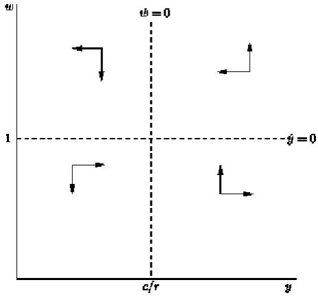
𝑤̇ = 𝑤(−𝑐 + 𝑟𝑦) (2)

The first equation captures the profit squeeze theory and the second the reserve army effect. A number of simplifying modifications are made to the original Goodwin model. In the original, it is assumed that both labour productivity and the labour force increase at steady exogenously determined rates. In our formulation we assume that these remain constant. Our model thus generates cycles in output around the steady state, while the original is a growth model. We replace employment (in the original model) with output; since Goodwin assumes a fixed marginal product of labour (a Leontieff production function) and an elastic supply of labour this makes no difference to the logic of the system.

Figure 1. Phase diagram for the Goodwin Model

The Goodwin system specified in equations (1) and (2) has two stationary points, the first where both variables are equal to zero, and the second at,

𝑦∗₌𝑐

𝑟, 𝑤∗= 1

The first stationary point can be shown to be an unstable saddle-point, while the second is the centre of a family of concentric closed orbits (for a proof, see Goodwin, 1967). The shapes of the orbits are defined by the parameters of the model, while the specific orbit generated by the system is determined by the starting values of the variables. The phase diagram for the model is shown in Figure 1 and the Jacobian matrix of the system evaluated at the non-zero stationary point is the following,

5 𝐽 = [0 −

𝑐 𝑟

𝑟 0 ] = [0 −+ 0]

The non-zero stationary point occurs at the intersection of the two nullclines of the system: 𝑦 =𝑐_𝑟 and 𝑤 = 1. The model generates cyclical dynamics because the off-axis entries have different signs. The direction of rotation is determined by the order in which the signs of the off-axis entries appear. In the current system, the direction of rotation is counter-clockwise in (𝑦, 𝑤) space: output peaks before the wage share.

It should be noted that - as in Goodwin’s original - our model is specified so that the wage share is not bounded and, in particular, may exceed unity. We have chosen this specification for the sake of simplicity. As shown by Desai et. al (2006), replacing the linear functions of the Goodwin model with suitable non-linear alternatives transforms the model so that employment rates and the wage share remain within the range (0,1). While we use the linear version of the model for the sake of clarity, this means that the absolute values of variables should not be seen as meaningful – our primary interest is in the dynamics of motion.

The Goodwin model has given rise to a rich literature. This comprises both more elaborate cyclical models (e.g. Skott 1989, Shah and Desai 1981) and empirical research which either looks for the existence of Goodwin-like patterns in historical data or estimates the behavioural relationships of cyclical models. An early debate in the Marxian literature focused on the mechanisms driving post-war US business cycles. One side of the debate followed Goodwin in arguing the upper turning point arises from a profit squeeze due to rising wages (e.g. Goldstein, 1999a, 1999b, 2002). The other argued that insufficient aggregate demand is the primary cause of downturns (e.g. Sherman, 1997, Van Lear 1999).

More recently, there has been debate among those inspired by the Goodwin literature and those who emphasise the role of aggregate demand. The followers of Goodwin argue that graphical plots of the wage share and unemployment show counter-clockwise patterns consistent with the

dynamics of the Goodwin model. This literature distinguishes between long-run and short-run cycles. Solow (1990) examines the data and concludes that there is very weak evidence for long-run Goodwin cycles. Flaschel et al. (2010), update previous research by Flaschel and Groh (1995) and examine data for eight OECD countries, concluding there is strong evidence for a long-run Goodwin cycle. Veneziani and Mohun (2006) argue that such long-run cycles are theoretically problematic and the empirical trends are more likely to be driven by structural change. The evidence for shorter-run Goodwin cycles (of 10-15 years duration) appears stronger. Desai (1984) presents evidence of such cycles in the post-war UK. Harvie (2000) examines data from 10 OECD countries, finding evidence of incomplete (approximately three-quarter-length) Goodwin cycles in most of the countries examined. Mohun and Veneziani (2008) find strong evidence for short-run Goodwin cycles in the post-war US data.

6 distribution and profit rates, regimes can be classified as either wage-led or profit-led. The

connection with the Goodwin model stems from Goodwin’s assumption of a profit-led regime – a wage-led regime will not, in general, generate anti-clockwise cycles. Hein and Vogel (2008), Naastepad and Storm (2006), Onaran and Galanis (2014), Stockhammer et al (2009), and

Stockhammer and Stehrer (2011) estimate consumption, investment and net export equations and find that aggregate demand is wage-led in many countries. On the other hand, Barbosa-Filho and Taylor (2006) and Flaschel and Proano (2007) estimate demand and distribution equations and find evidence that demand in the USA is profit-led.3 Kiefer and Rada (2015) do so for a panel of OECD countries with a set of control variables that shift income distribution and find that demand is profit led.

A recent contribution by Taylor (2012) connects the theoretical and empirical strands. Taylor contrasts two models of distribution and demand. The first combines a locally stable “Domar-style” investment function (that leads to a profit-led regime) with a Goodwin-type reserve-army

distribution function. This is contrasted with a model which combines an unstable “Harrod-style” investment function (which produces a wage-led demand regime) with a distribution function based on a pro-cyclical profit-share. The first model generates Goodwin-type counter-clockwise cycles in output-distribution space, while the second generates cycles which turn in the opposite direction. On the basis of the empirical evidence, Taylor argues that the anticlockwise Goodwin-type

movement is what is being observed. He concludes, “Overall, Domar-style investment and a profit squeeze appear to fit the data better than Harrod and short-run wage-led aggregate demand” (p. 50). Taylor thus cites the apparent existence of counter-clockwise cycles in the empirical data as evidence for a Goodwin mechanism and a profit-led demand regime. A similar approach is taken by Diallo et al (2011) who construct a model with four possible regimes: clockwise and counter-clockwise cyclical regimes, and two saddle-point cases which do not generate cyclical behaviour. Diallo et al (2011) also conclude that the empirical evidence supports the profit-led version of the model.

Taylor extends the analysis by discussing models where cyclical behaviour is generated by the interaction of financial variables and demand in a Minskian framework in which asset prices and debt interact. However, these financial models are left only partially specified. In particular, the role of income distribution is not investigated, thus the question what type of cycles the financial group of models gives rise to in the wage share-income space is not investigated.

It is this question that we consider in the remainder of the paper. In particular, we take issue with the claim that finding something that looks like Goodwin cycles in the data implies that the

mechanism generating those cycles is a profit-led demand regime. We demonstrate that such cycles can instead be generated by the interaction of financial fragility, demand and distribution. In

3

7 particular, models can be constructed which generate Goodwin-type cycles but do not rely on a profit-led demand function.

A Minsky model

Unlike the Goodwin model, there is no canonical version of the Minsky cycle. Minsky’s own work (Minsky 1975, 1986) presents a verbal description of the cycle mechanism, but no formal model. Consequently, several different models purporting to summarise his argument have been proposed (e.g. Skott 1994, Asada 2001, Fazzari et al 2008, Charles 2008). For our purposes, however, the basic structure of the argument is clear enough. The cycle results from the interaction of goods market demand and financial fragility of non-financial businesses.

This section will present only a minimalistic version of the Minsky model – the main aim of the paper is to investigate the properties of the model when it is extended to include a reserve army function. To ensure comparability with the structure of the Goodwin we also use a predator-prey model. The model consists of two differential equations:

𝑓̇ = 𝑓(−1 + 𝑝𝑦) (3)

𝑦̇ = 𝑦(1 − 𝑓) (4)

Equation (3) specifies the rate of increase of financial fragility, f, as a positive function of the level of demand. The assertion is that during a boom firms adopt a progressively more optimistic outlook and therefore take on higher levels of debt (relative to revenue) – financial fragility is usually thought of as the inverse of the debt-to-income ratio of firms. Banks share the optimistic outlook and are increasingly willing to lend as the boom progresses. The balance sheets of economic units in the Minsky model endogenously become more fragile at higher levels of output.

Equation (4) specifies an inverse relationship between aggregate demand growth and the degree of fragility of the system.This is because the degree of indebtedness of firms makes them vulnerable to bankruptcy once interest rates rise and a larger share of cash flows is absorbed by debt services, which negatively affects investment. Skott (1994), Asada (2001), Fazzari et al (2008), and Charles (2008) derive such models from behavioural functions and discuss them further.

8 investment of firms. In such a framework, it is not clear why the debt ratio should rise during the boom. Rather, the high rate of investment growth during the boom should lead to decreasing leverage ratios. 4 Our model avoids both issues by design.

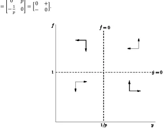
First, Equation 3 states that financial fragility increases with output, following Minsky’s argument that the leverage ratio is pro-cyclical. Second, Equation 4 does not specify the mechanism which leads to the upper turning point, such as a rise in interest rate). Rather it simply posits that higher fragility leads to lower growth of demand. The phase diagram for the model is shown in Figure 2. The non-trivial steady state solution of the Minsky model is

𝑓∗_{= 1, 𝑦}∗₌ 1 𝑝

and the Jacobian at the steady state is

𝐽 = [₋01 𝑝 𝑝 0] = [

0 + − 0].

Figure 2 Phase diagram for Minsky model

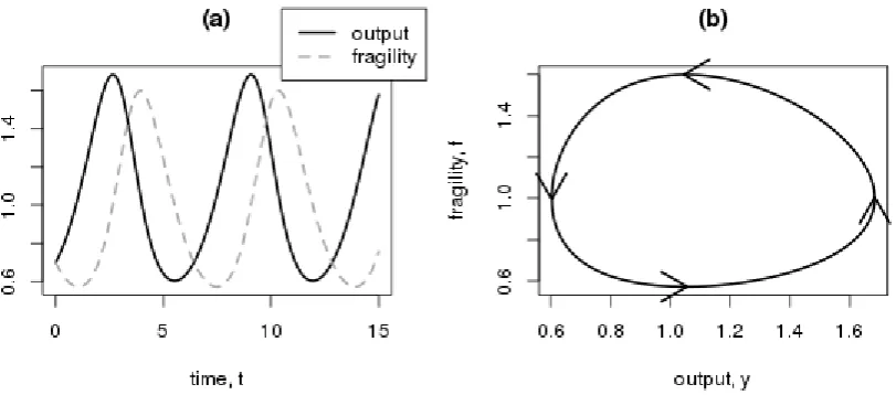
Figure 3 simulates the dynamics of the system with 𝑝 = 0.95 and initial values 𝑦 = 0.7, 𝑓 = 0.7. The system generates cycles such that peaks in output precede peaks in financial fragility (Figure 3a).

9 Alternatively, this could be expressed by saying that the system produces anti-clockwise motion in output-fragility space (Figure 3b).

Figure 3 Simulation of Minsky model

A Minsky model with a reserve army effect

In this section we discuss a Minsky model that includes a reserve army effect. The dynamics of this system will be driven entirely by the interaction between financial fragility and demand. The distribution function has, by design, no feedback on demand. We retain equations 3 and 4. To this we add a distribution equation with a reserve army effect:

𝑤̇ = 𝑤(−𝑐 + 𝑟𝑦 − 𝑤) (5)

This equation is similar to Equation (2), but additionally includes a negative own-feedback term. This may be interpreted as representing mechanisms which counteract workers’ wage demands.

Intuitively, wages will also be affected factors like the organisational strength of unions or supply-side factors such a labour productivity. These mechanisms become progressively stronger at higher real wages, placing an effective upper bound on the wage share. The mathematical formulation is equivalent to what is known as the logistic equation in biology. In the context of population dynamics, the logistic equation imposes an upper bound on the population due to the carrying capacity of the environment (Nolting et al. 2008).

10 the population of another species, but the causality is unidirectional (Chauvet et al. 2002, Nolting et al. 2008).5

This model may appear similar to models that try to integrate Goodwin and Minsky mechanisms, such as Keen (1995). However, there is an important difference in terms of the synthesis as well as in terms of the questions these models are intended to answer. Keen (1995) constructs a model with the intention of examining the properties of models which have feedbacks from both distribution and finance to aggregate demand. Causality thus runs from both demand and distribution to finance and vice versa. We are asking a different question. We are interested (in this section) in a model that has a Minsky cycle and a Marxian distribution function but has no feedback from distribution to demand.6 We subsequently extend the analysis to allow for feedback from distribution to demand. The interior steady state of the model occurs at the following point:

𝑓∗_{= 1, 𝑦}∗₌1

𝑝, 𝑤∗= −𝑐 + 𝑟 𝑝.

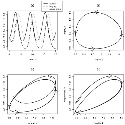
The dynamics of the model are simulated with parameters 𝑐 = 1, 𝑝 = 0.95, 𝑟 = 1.6 and starting values of 𝑓 = 0.7, 𝑦 = 0.7, 𝑤 = 0.8. The model generates oscillations in all three variables (Figure 4a). Peaks in output precede those in fragility and the wage share. As in the pure Minsky model, the cycle that drives the system is generated by the interaction between fragility and demand (Figure 4b; a formal analysis of stability conditions is delegated to Appendix A.1).

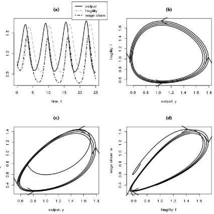
The key feature of this system is that it generates limit cycles in 𝑦 and 𝑤 that look like a Goodwin cycle (Figure 4c).7 This cycle, however, is simply a side effect of the cycle generated by the interaction of financial fragility and demand. We call this a pseudo-Goodwin cycle: a

counter-clockwise rotation in (𝑦, 𝑤) space that is not due to the mechanisms of the original Goodwin model.8 The model also generates cycles in distribution and fragility. Like the pseudo-Goodwin cycles these do not arise out of direct causal links between these variables but as side effects of other causal relations.

5 _{Strictly speaking a scavenger population depends on deaths of prey, i.e. the kill rate. Our wage share depends}

on the population of output rather than its death rate. Biologically speaking distribution thus plays the role of a harmless parasite rather than a scavenger.

6 _{We are bypassing the issue of whether income distribution can have an effect on financial fragility. As in}

other post-Keynesian models, changes in the wage share have conflicting effects on aggregate demand because they affect consumption and investment in opposite directions. Retained (realised) profits will affect financial fragility if it is defined as the debt to income ratio of business. An exploration of this interesting issue is beyond the scope of this paper.

7 _{This occurs when} 1

𝑝≥ 𝑐

𝑟. If this condition does not hold the system generates damped cycles. 8

11 If Equation (5) is replaced with Equation (2) so that the wage share is not bounded, the system will still exhibit pseudo-Goodwin cycles – anticlockwise oscillations in (𝑦, 𝑤) space. The model will, however, in general not generate limit cycles in (𝑦, 𝑤) space.9 Instead, we obtain either damped or explosive oscillations in distribution. The behaviour of the system is determined by the value of 1

𝑝− 𝑐

𝑟. If this expression is negative, the system generates damped oscillations in 𝑤 so that the wage share eventually falls to zero. Intuitively this corresponds to a case in which falls in the wage share during recessions exceed increases during booms so that the wage share exhibits a secular declining trend. In the case that 1_𝑝−𝑐_𝑟 is positive we get oscillations with increasing amplitude. Intuitively this represents a case in which the wage share rises further during booms than it falls during recessions, resulting in a tendency towards a long-run increase in the wage share.

9 _{A closed orbit in distribution and output is possible if} 1

12

Figure 4 Simulation of Minsky model with reserve army effect

A Minsky model with reserve-army effect and a wage-led effect in the demand function

The previous section demonstrates that pseudo-Goodwin cycles can arise in a system in which income distribution has no influence on demand. In this section we introduce one more ingredient into our model: a positive feedback from the wage share to output. In other words, we investigate whether a pseudo-Goodwin cycle can arise in wage-led economy.

To do so, we retain equations (3) and (5) but replace Equation (4) with Equation (6), which includes a positive feedback from the wage share to demand.

𝑦̇ = 𝑦(1 − 𝑓 + 𝑠𝑤) (6)

13 𝑦∗₌1

𝑝, 𝑓

∗_{= 1 + 𝑠 (−𝑐 +}𝑟 𝑝) , 𝑤

∗_{= −𝑐 +}𝑟 𝑝.

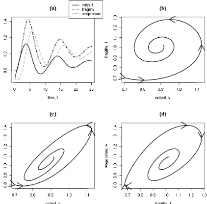
The dynamics of this system are depicted in Figure 5, assuming parameter values of 𝑐 = 1, 𝑝 = 0.95, 𝑟 = 1.6, 𝑠 = 0.02 and starting values 𝑓 = 0.7, 𝑦 = 0.7, 𝑤 = 0.8. The cyclical behaviour of the model is still driven by the interaction between 𝑦 and 𝑓 (Figure 5b). However, this no longer produces a closed orbit because of the instability introduced by the wage-led demand term (for a proof of the existence of explosive cycles see Appendix A.2). As before, if f were fixed, the system in (6) and (5) would exhibit explosive non-oscillatory growth: the feedback from distribution to output as well as from output to distribution are positive.

Figure 5c shows that our model still exhibits the key feature of a pseudo-Goodwin cycle – counter-clockwise motion in output-wage share space. The cyclical motion is now unstable, so that outward spirals are generated in the phase space of all three pairs of variables. The introduction of a wage-led demand function into the system does not prevent the generation of pseudo-Goodwin cycles.10 Instead it simply switches the system from generating limit cycles to unstable oscillations. Evidence of counter-clockwise motion in output-wage-share space does not therefore provide sufficient evidence to rule out a wage-led demand regime.

14

Figure 5 Simulation of Minsky model with reserve army effect and wage-led demand.

15 A more complex system: a generalised Minsky model with reserve army distribution and wage-led demand

Up to this point, we have intentionally kept our models as simple as possible, in order to demonstrate our key point that any business cycle system featuring a reserve-army distribution function can generate Goodwin-like cycles – regardless of the specification of the demand function. In this section we present a more general, fully parameterised system in which all three equations include negative own-feedback terms. In biology, similar specifications are used to represent within-species competition, placing limits, for example, on the environmental carrying capacity of a prey species in the absence of a predator. With the inclusion of these terms, the system can generate either stable or unstable dynamics, depending on parameter values.

In economic terms, these negative own-feedback effects reduce the tendency for variables to grow without limits and serve to damp the oscillations of the system. In the demand function such effects may be due to counter-cyclical government intervention or supply-side shortages exerting a

stabilising effect on the system during the boom (Taylor 2012) discusses such a feedback in the investment function as ‘Domar-type’.11 Equation 7 introduces such an effect. We assume, likewise, that growth of both the wage share and financial fragility are damped as their levels increase (equations 8 and 9). The wage share could be affected by the organisational strength of labour and capital and financial fragility will be contained by financial regulation.

Formally, the system is expressed as follows

𝑓̇ = 𝑓(−𝑎 + 𝑝𝑦 − 𝑘𝑓) (7)

𝑦̇ = 𝑦(𝑏 − 𝑞𝑓 + 𝑠𝑤 − ℎ𝑦) (8)

𝑤̇ = 𝑤(−𝑐 + 𝑟𝑦 − 𝑔𝑤) (9)

The non-trivial fixed points of this system are

𝑓∗₌−𝑎 + 𝑝𝑦∗ 𝑘

𝑦∗₌𝑏 + 𝑎𝑞

𝑘 −𝑠𝑐𝑔 ℎ +𝑝𝑎_{𝑘 −}𝑟𝑠_𝑔

𝑤∗₌−𝑐 + 𝑟𝑦∗ 𝑔

This system is capable of producing a wide range of behaviours and the stability conditions are significantly more complex than for the models presented in previous sections. An exhaustive analysis is beyond the scope of the paper, but we will highlight some key features and explore some properties based on numerical simulations.

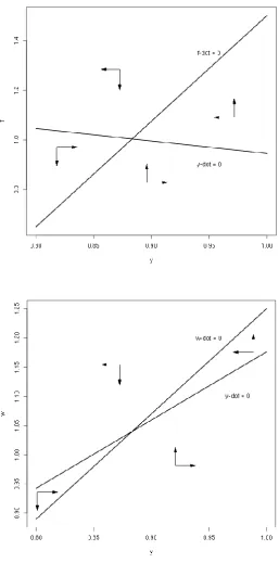
16 An important feature of this model is that the steady-state level of output now depends on the parameters of the wage equation, whereas it was independent in the simpler model of the previous section. In other words, the nullclines are sloped. This is illustrated in Figure 6. Figure 6.a shows the nullclines of 𝑓 and 𝑦, holding 𝑤 constant. Figure 6.b shows nullclines of 𝑤 and 𝑦 holding 𝑓

constant.12 The slope of the nullclines can be interpreted as describing long run relationships, while the points of intersection occur at the steady state. The current model is thus wage led in the long run while higher levels of financial fragility are associated with lower output.13

12 _{The parameters used to generate Figures 6 and 7 are the following: 𝑎 = 0.55, 𝑏 = 0.7, 𝑐 = 0.55, 𝑝 =} 0.85, 𝑞 = 0.7, 𝑟 = 1.8, 𝑠 = 0.3, 𝑘 = 0.2, ℎ = 0.35, 𝑔 = 1.

17

Figure 6 Nullclines and phase diagram for generalised Minksy model

18

Figure 7 Simulation of generalised Minsky model with weak wage-led effect

This model does not, however, always produce damped cycles. With a stronger wage-led component in the demand function (i.e. an increase in the parameter 𝑠), as shown in Figure 8, the model can produce explosive dynamics, as with the simpler model in the previous section.14 While a full analysis of the properties of the system is beyond the scope of the paper, simulations make clear that the relative size of the wage-led effect compared to the stabilising feedback effects is one of the factors determining the stability of the system. Negative self-feedback effects stabilise the system. Thus, under certain parameter combinations, the model can generate pseudo-Goodwin cycles in a wage-led Minsky model without producing system-wide instability. Again, the inclusion of the wage wage-led element in the demand function does not alter the direction of the cycle in 𝑤, 𝑦 space, but does

19 affect stability.15 The model will produce explosive behaviour if the wage-led effect is large relative to the self-stabilising forces. Overall, our findings for the extended Minsky model with wage led demand are consistent with the simpler models of the previous sections in that pseudo-Goodwin cycles can arise despite wage-led demand regimes. We also confirm that wage-led demand can lead to explosive dynamics but this is a possible, not necessary, outcome.

Figure 8. Simulation of generalised Minsky model model with strong wage-led effect

20 Conclusion

Goodwin’s (1967) model generates counter-clockwise cycles in output-wage-share space due to the interaction of a profit-led demand regime and a reserve army distribution function. The paper has demonstrated that counter-clockwise cycles in output-wage-share space can arise for reasons that are unrelated to the Goodwin mechanism. We call such cycles pseudo-Goodwin cycles. As an illustration, a Minsky model of the interaction of financial fragility and output is extended to include a reserve army function. In a second step we introduce a wage-led effect in the demand equation. In both cases we show that pseudo-Goodwin cycles can arise. A more complex model demonstrates that such cycles can also be generated in a system which also has ‘long-run’ wage led features, i.e. a system in which a higher wage share is associated with higher steady-state output. The wage-led demand regime in conjunction with a reserve army distribution function does constitute a force for long-run instability of the system. In a more complex version of the model either stable or unstable dynamics can arise depending on the size of the wage-led demand effect relative to the self-stabilising forces of the system.

This leads to the following conclusions. First, any system which generates cycles in output alongside a reserve army distribution mechanism behaviour will produce pseudo-Goodwin cycles so long as there is no a feedback mechanism from income distribution. Even in the case of a wage-led demand effect, pseudo-Goodwin cycles are possible. Second, the existence of a counter-clockwise movement of in output wage share space is therefore not a sufficient condition for the existence of actual Goodwin cycles and can therefore not be interpreted as prima facie evidence for the existence of a profit-led demand regime. Rather, a wage-led demand regime can be perfectly consistent with pseudo-Goodwin cycles.

References

Asada, T. 2001. Nonlinear dynamics of debt and capital: a Post-Keynesian analysis. In Y. Aruka (Ed.)

Evolutionary Controversies in Economics (Tokyo: Springer-Verlag).

Barbosa-Filho, N., 2015, Elasticity of substitution and social conflict: a structuralist note on Piketty’s

Capital in the Twenty-first Century, Cambridge Journal of Economics, Advance Access.

Barbosa-Filho, N., and Taylor, L. 2006. Distributive and demand cycles in the US economy – a structuralist Goodwin model. Metroeconomica 57, (3): 389-411

Charles, S., 2008. Teaching Minsky’s financial instability hypothesis: a manageable suggestion.

Journal of Post Keynesian Economics 31, 1: 125-38

Chauvet, E., Paullet, J., Previte, J. and Walls, Z. 2002. A Lotka Volterra three-species food chain.

Mathematics Magazine 75, 4: 253-55

21 Diallo, M., Flaschel, P., Krolzig, H. and Proaño, C., 2011. Reconsidering the dynamic interaction between real wages and macroeconomic activity. Research in World Economy. 2, 1, 77-93 Fazzari, S., Ferri, P. and Greenberg, E., 2008. Cash flow, investment, and Keynes–Minsky cycles.

Journal of Economic Behavior and Organization, 65, 3–4, 555–572

Flaschel, P., and Groh, G. 1995. The classical growth cycle: reformulation, simulation and some facts.

Economic Notes, 24, 293–326.

Flaschel, P., Groh, G., Kauermann, G., and Teuber T. 2010. The Goodwin Distributive Cycle After Fifteen Years of New Observations, in Flaschel, P. (ed.), Topics in Classical Micro- and

Macroeconomics, Springer Berlin Heidelberg

Flaschel, P. and Proaño C. 2007. AS-AD Disequilibrium dynamics and the Taylor interest rate policy rule: Euro-Area based estimation and simulation. In: Aspects of Modern Monetary and

Macroeconomic Policies. Ed. P. Arestis, E. Hein and E. Le Heron. Houndsmill: Palgrave MacMillan Goldstein, J. P. 1999a. Predator-Prey Model Estimates of the Cyclical Profit Squeeze.

Metroeconomica 50, 2, pp. 139-173.

Goldstein, J.P. 1999b. The simple analytics and empirics of the cyclical profit squeeze and cyclical underconsumption theories: clearing the air. Review of Radical Political Economics, 1999, 31(2), pp. 74–88

Goldstein, J. P. 2002. The profit squeeze is supported by the PW cycle indicator. Review of Radical Political Economics, 34, 75–77.

Goodwin, R.M., 1967. A Growth Cycle, in C.H. Feinstein, editor, Socialism, Capitalism and Economic Growth. Cambridge: Cambridge University Press

Goodwin, R.M. 1972, A Growth Cycle, in Hunt, E.K. and Schwartz, J.G. (eds.), A Critique of Economic Theory. Harmondsworth: Penguin (revised version of Goodwin, 1967)

Harvie, D. 2000. Testing Goodwin: growth cycles in ten OECD economies. Cambridge Journal of Economics 24: 349-76

Hein, E., and Vogel, L. 2008. Distribution and growth reconsidered – empirical results for six OECD countries, Cambridge Journal of Economics, 32: 479-511.

Keen, S. 1995. Finance and economic breakdown modelling Minsky’s ‘financial instability hypothesis,’ Journal of Post Keynesian Economics, 17, pp. 607–635.

Kiefer, D, and Rada, C, 2015. Profit maximizing goes global: the race to the bottom Cambridge Journal of Economics 39 (5): 1333-1350

Lavoie, M. and Seccareccia, M. 2001. Minsky’s financial Fragility Hypothesis: A Missing

22 Michell, J. 2014a. Speculation, financial fragility and stock-flow consistency, in The Great Recession and the contradictions of contemporary capitalism, R. Bellofiore and G. Vertova (eds.), Edward Elgar. Michell, J. 2014b. A Steindlian account of the distribution of corporate profits and leverage: A stock-flow consistent macroeconomic model with agent-based microfoundations, Post Keynesian

Economics Study Group Working Paper PKWP1412

Minsky, H. 1975. John Maynard Keynes, New York: Columbia University Press Minsky, H.1986. Stabilizing an unstable economy. New Haven: Yale University Press Mohun, S, and Veneziani R. 2008. Goodwin Cycles and the U.S. Economy 1948-2004. In:

Mathematical Economics and the Dynamics of Capitalism, ed. P. Flaschel and M. Landesmann. Routledge, 2008. Chapter 6, pp.107-130

Naastepad, C.W.M., and Storm S. 2006/7. OECD demand regimes (1960-2000). Journal of Post-Keynesian Economics, 29: 213-248.

Nolting, B, Paullet, J, and Previte, J. 2008. Introducing a scavenger onto a predator prey model.

Applied Mathematics E-Notes 8, 214-22

Onaran, Ö., Galanis, G. 2014, "Income distribution and growth: a global model" Environment and Planning A46(10) 2489–2513

Shah, A. and Desai, M. 1981, Growth cycles with induced technical change, The Economic Journal , Vol. 91, No. 364 (Dec.) , pp. 1006-1010.

Sherman, H. 1979. A Marxist theory of the business cycle. Review of Radical Political Economics, 11, 1–23.

Sherman, H. 1997. Theories of cyclical profit squeeze. Review of Radical Political Economics, 29, 139– 147.

Solow, R. M. 1990. Goodwin’s growth cycle: reminiscence and rumination. In K. V. Velupillai (Ed.)

Multisectoral Macrodynamics. London: Macmillan.

Stockhammer, E. 2004. Is there an equilibrium rate of unemployment in the long run? Review of Political Economy: 16 (1) 59-77

Stockhammer, E., Onaran Ö. and Ederer S. 2009. Functional income distribution and aggregate demand in the Euro area. Cambridge Journal of Economics: 33 (1): 139-159

Stockhammer, E, Stehrer, R. 2011. Goodwin or Kalecki in demand? Functional income distribution and aggregate demand in the short run. Review of Radical Political Economics 43(4), 506–522 Skott, P. 1989. Effective demand, class struggle and cyclical growth. International Economic Review, 30, 1 , pp. 231-247

23 Taylor, L. 2012. Growth cycles, asset prices and finance. Metroeconomica 63, 1: 40-63

Veneziani, R. and Mohun, S. 2006. Structural stability and Goodwin’s growth cycle, Structural Change and Economic Dynamics, 17, pp. 437—451.

Volterra, V. 1926. Variazioni e fluttuazioni del numero d’individui in specie animali conviventi, Mem. Accademia die Lincei, Roma, 2, 31--113

24 Appendix

A.0 Routh Hurwitz stability conditions for a three-dimensional system

Given a three dimensional Jacobian of the form,

𝐽3𝐷= [

𝐽₁₁ 𝐽₁₂ 𝐽₁₃ 𝐽₂₁ 𝐽₂₂ 𝐽₂₃ 𝐽31 𝐽32 𝐽33 ]

The characteristic equation of this system is: 𝑞3_{+ 𝑎}

1𝑞2+ 𝑎2𝑞 + 𝑎3

Where

𝑎1 = −𝑇𝑟(𝐽3𝐷) = −(𝐽11+ 𝐽22+ 𝐽33)

𝑎₂= sum of all principal second-order minors of 𝐽3𝐷 = |𝐽_𝐽11 𝐽12

21 𝐽22| + |

𝐽11 𝐽13

𝐽₃₁ 𝐽₃₃| + |𝐽𝐽22₃₂ 𝐽𝐽23₃₃|

𝑎3= −𝐷𝑒𝑡(𝐽3𝐷)

For this system to be stable, the following must hold: 𝑎₁, 𝑎₂, 𝑎₃> 0

𝑏 = 𝑎₁𝑎₂− 𝑎3 > 0

A.1 Stability analysis for Minsky model with reserve army effect

The model is comprised of equations (3), (4) and (5), reproduced here for ease of exposition.

𝑓̇ = 𝑓(−1 + 𝑝𝑦) (3)

𝑦̇ = 𝑦(1 − 𝑓) (4)

𝑤̇ = 𝑤(−𝑐 + 𝑟𝑦 − 𝑤) (5)

The non-zero steady state of the system occurs where, 𝑓∗_{= 1, 𝑦}∗₌1

𝑝, 𝑤∗= 𝑟 𝑝− 𝑐

25 𝐽 = [

−1 + 𝑝𝑦

𝑝𝑓

−𝑦

1 − 𝑓

0 𝑟𝑤 −𝑐 + 𝑟𝑦 − 2𝑤

]

Evaluated at the non-zero steady state,

𝐽∗_{= [}

0

𝑝𝑓

∗ ₀

−𝑦

0 𝑟𝑤∗ _−𝑤∗

]

The Routh-Hurwitz conditions specified in Appendix A.0 can be calculated as follows, 𝑎₁= −(0 + 0 − 𝑤∗_{) = 𝑤}∗

𝑎₂= (0 − −(𝑝𝑓∗_𝑦∗_{)) + (0 − 0) + (0 − 0) = 1}

𝑎₃= − ( −𝑝𝑓∗₍₋1

𝑝⋅ −𝑤∗)) = 𝑤∗

𝑏 = 𝑎1𝑎2− 𝑎3= 0

A.2 Stability of Minsky model with reserve army effect and wage-led demand

If we take the system analysed in Appendix A.1, and replace equation (4) with (4’),

𝑦̇ = 𝑦(1 − 𝑓 + 𝑠𝑤) (4’)

We obtain the augmented Minsky system with reserve army mechanism and wage-led demand. In this case, the Routh-Hurwitz conditions become the following:

𝑎₁= 𝑤₀

𝑎₂= 1 + 𝑠𝑤₀(1 −𝑟 𝑝)

𝑎₃= 𝑤₀(1 + 𝑠𝑤0)

𝑏 = 𝑤₀(𝑓₀−𝑠𝑟𝑤0

𝑝 ) − 𝑓0𝑤0

= −𝑠𝑟𝑤0 𝑝

The non-zero fixed point cannot be stable since 𝑎1 and 𝑏 cannot simultaneously be positive. If 𝑠 > 0 then if _𝑝1>𝑐_𝑟, so that 𝑤0> 0 then 𝑏 < 0. In this case, the system is unstable, and generates