From Global to Local Similarities: A Graph Based Contextualization Method using Distributional Thesauri

From Global to Local Similarities:

A Graph-Based Contextualization Method using Distributional Thesauri

Chris Biemann and Martin Riedl

Computer Science Department, Technische Universit¨at Darmstadt Hochschulstrasse 10, D-64289 Darmstadt, Germany

{riedl,biem}@cs.tu-darmstadt.de

Abstract

After recasting the computation of a distribu-tional thesaurus in a graph-based framework for term similarity, we introduce a new con-textualization method that generates, for each term occurrence in a text, a ranked list of terms that are semantically similar and compatible with the given context. The framework is in-stantiated by the definition of term and con-text, which we derive from dependency parses in this work. Evaluating our approach on a standard data set for lexical substitution, we show substantial improvements over a strong non-contextualized baseline across all parts of speech. In contrast to comparable approaches, our framework defines an unsupervised gener-ative method for similarity in context and does not rely on the existence of lexical resources as a source for candidate expansions.

1 Introduction

Following (de Saussure, 1916) we consider two dis-tinct viewpoints: syntagmaticrelations consider the assignment of values to a linear sequence of terms, and theassociative (also: paradigmatic)viewpoint assigns values according to the commonalities and differences to other terms in the reader’s memory. Based on these notions, we automatically expand terms in the linear sequence with their paradigmati-cally related terms.

Using the distributional hypothesis (Harris, 1951), and operationalizing similarity of terms (Miller and Charles, 1991), it became possible to compute term similarities for a large vocabulary (Ruge, 1992). Lin (1998) computed adistributional thesaurus (DT) by comparing context features de-fined over grammatical dependencies with an ap-propriate similarity measure for all reasonably fre-quent words in a large collection of text, and evalu-ated these automatically computed word similarities

against lexical resources. Entries in the DT consist of a ranked list of the globally most similar terms for atarget term. While the similarities are dependent on the instantiation of the context feature as well as on the underlying text collection, they are global in the sense that the DT aggregates over all occurrences of target and its similar elements. In our work, we will use a DT in a graph representation and move from a global notion of similarity to a contextual-ized version, which performs context-dependent text expansion for all word nodes in the DT graph.

2 Related Work

The need to model semantics just in the same way as local syntax is covered by the n-gram-model, i.e. trained from a background corpus sparked a large body of research on semantic modeling. This in-cludes computational models for topicality (Deer-wester et al., 1990; Hofmann, 1999; Blei et al., 2003), and language models that incorporate topical (as well as syntactic) information, see e.g. (Boyd-Graber and Blei, 2008; Tan et al., 2012). In the Computational Linguistics community, the vector space model (Sch¨utze, 1993; Turney and Pantel, 2010; Baroni and Lenci, 2010; Pucci et al., 2009; de Cruys et al., 2013) is the prevalent metaphor for representing word meaning.

While the computation of semantic similarities on the basis of a background corpus produces a global model, which e.g. contains semantically similar words for different word senses, there are a num-ber of works that aim at contextualizing the infor-mation held in the global model for particular oc-currences. With his predication algorithm, Kintsch (2001) contextualizes LSA (Deerwester et al., 1990) for N-VP constructions by spreading activation over neighbourhood graphs in the latent space.

In particular, the question of operationalizing se-mantic compositionality in vector spaces (Mitchell

and Lapata, 2008) received much attention. The lex-ical substitution task (McCarthy and Navigli, 2009) (LexSub) sparked several approaches for contextual-ization. While LexSub participants and subsequent works all relied on a list of possible substitutions as given by one or several lexical resources, we de-scribe a graph-based system that is knowledge-free and unsupervised in the sense that it neither requires an existing resource (we compute a DT graph for that), nor needs training for contextualization.

3 Method

3.1 Holing System

For reasons of generality, we introduce the holing operation (cf. (Biemann and Riedl, 2013)), to split any sort of observations on the syntagmatic level (e.g. dependency relations) into pairs of term and context features. These pairs are then both used for the computation of the global DT graph similarity and for the contextualization. This holing system is the only part of the system that is dependent on a pre-processing step; subsequent steps operate on a unified representation. The representation is given by a list of pairs<t,c>wheretis the term (at a cer-tain offset) andcis the context feature. The position oftincis denoted by a hole symbol ’@’. As an ex-ample, the dependency triple(nsub;gave2;I1)

could be transferred to<gave2,(nsub;@;I1)>

and<I1,(nsub;gave2;@)>.

3.2 Distributional Similarity

Here, we present the computation of the distribu-tional similarity between terms using three graphs. For the computation we use the Apache Hadoop Framework, based on (Dean and Ghemawat, 2004). We can describe this operation using a bipartite ”term”-”context feature” graph T C(T, C, E) with

T the set terms, C the set of context features and

e(t, c, f) ∈ E edges between t ∈ T, c ∈ C

with f = count(t, c) frequency of co-occurrence. Additionally, we define count(t) and count(c) as the counts of the term, respectively as the count of the context feature. Based on the graph T C

we can produce a first-order graph F O(T, C, E), with e(t, c, sig) ∈ E. First, we calculate a signif-icance scoresig for each pair(t, c) using Lexicog-rapher’s Mutual Information (LMI): score(t, c) =

LM I(t, c,) = count(t, c) log₂(_{count(t)count(c)}count(t,c) )

(Evert, 2004). Then, we remove all edges with

score(t, c) < 0 and keep only the p most signif-icant pairs per term t and remove the remaining edges. Additionally, we remove features which co-occur with more then 1000 words, as these features do not contribute enough to similarity to justify the increase of computation time (cf. (Rychl´y and Kil-garriff, 2007; Goyal et al., 2010)). The second-order similarity graph between terms is defined as

SO(T, E) fort1, t2 ∈ T with the similarity score

s = |{c|e(t1, c) ∈ F O, e(t2, c) ∈ F O}|, which is

the number of salient features two terms share. SO

defines a distributional thesaurus.

In contrast to (Lin, 1998) we do not count how of-ten a feature occurs with a term (we use significance ranking instead), and do not use cosine or other sim-ilarities (Lee, 1999) to calculate the similarity over the feature counts of each term, but only count sig-nificant common features per term. This constraint makes this approach more scalable to larger data, as we do not need to know the full list of features for a term pair at any time. Seemingly simplistic, we show in (Biemann and Riedl, 2013) that this mea-sure outperforms other meamea-sures on large corpora in a semantic relatedness evaluation.

3.3 Contextual Similarity

The contextualization is framed as a ranking prob-lem: given a set of candidate expansions as pro-vided by theSOgraph, we aim at ranking them such that the most similar term in context will be ranked higher, whereas non-compatible candidates should be ranked lower.

First, we run the holing system on the lexical material containing our target word tw ∈ T0 ⊆

T and select all pairs <tw,ci> ci ∈ C0 ⊆ C

that are instantiated in the current context. We then define a new graphCON(T0, C0, S)with con-text features ci ∈ C0. Using the second-order

similarity graph SO(T, E) we extract the top n

similar termsT0={ti, . . . , tn}⊆T from the

second-order graphSO for twand add them to the graph

CON. We add edges e(t, c, sig) between all tar-get words and context features and label the edge with the significance score from the first order graph

calcu-late a ranking score for each ti with the harmonic

mean, using a plus one smoothing: rank(ti) =

Q

cj(sig(ti,cj)+1)/count(term(cj))

P

cj(sig(ti,cj)+1)/count(term(cj))

(term(cj) extracts

the term out of the context notation). Using that ranking score we can re-order the entriest1, . . . , tn

according to their ranking score.

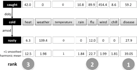
In Figure 1, we exemplify this, using the tar-get word tw= ”cold” in the sentence ”I caught a nasty cold.”. Our dependency parse-based

Figure 1: Contextualized ranking for target ”cold” in the sentence ”I caught a nasty cold” for the 10 most similar terms from the DT.

holing system produced the following pairs for ”cold”: <cold5 ,(amod;@;nasty4)>,

<cold5,(dobj;caught2;@)>. The top 10

candidates for ”cold” are T0={heat, weather, tem-perature, rain, flue, wind, chill, disease}. The scores per pair are e.g. <heat, (dobj;caught;@)>

with an LMI score of 42.0, <weather ,(amod;@;nasty)> with a score of 139.4. The pair <weather, (dobj;caught;@)>

was not contained in our first-order data. Ranking the candidates by their overall scores as given in the figure, the top three contextualized expansions are ”disease, flu, heat”, which are compatible with both pairs. For the top 200 words, the ranking of fully compatible candidates is: ”virus, disease, infection, flu, problem, cough, heat, water”, which is clearly preferring the disease-related sense of ”cold” over the temperature-related sense.

In this way, each candidate t’ gets as many scores as there are pairs containingc’in the holing system output. An overall score pert0 then given by the harmonic mean of the add-one-smoothed single scores – smoothing is necessary to rank candidates

t’that are not compatible to all pairs. This scheme

can easily be extended to expand all words in a given sentence or paragraph, yielding a two-dimensional contextualized text, where every (content) word is expanded by a list of globally similar words from the distributional thesaurus that are ranked according to their compatibility with the given context.

4 Evaluation

The evaluation of contextualizing the thesaurus (CT) was performed using the LexSub dataset, introduced in the Lexical Substitution task at Semeval 2007 (McCarthy and Navigli, 2009). Following the setup provided by the task organizers, we tuned our ap-proach on the 300 trial sentences, and evaluate it on the official remaining 1710 test sentences. For the evaluation we used the out of ten (oot) preci-sion and oot mode precipreci-sion. Both measures cal-culate the number of detected substitutions within ten guesses over the complete subset. Whereas en-tries in the oot precision measures are considered correct if they match the gold standard, without pe-nalizing non-matching entries, the oot mode preci-sion includes also a weighting as given in the gold standard1. For comparison, we use the results of the DT as a baseline to evaluate the contextualization. The DT was computed based on newspaper corpora (120 million sentences), taken from the Leipzig Cor-pora Collection (Richter et al., 2006) and the Giga-word corpus (Parker et al., 2011). Our holing system uses collapsed Stanford parser dependencies (Marn-effe et al., 2006) as context features. The contextual-ization uses only context features that contain words with part-of-speech prefixes V,N,J,R. Furthermore, we use a threshold for the significance value of the LMI values of 50.0, p=1000, and the most similar 30 terms from the DT entries.

5 Results

Since out contextualization algorithm is dependent on the number of context features containing the tar-get word, we report scores for tartar-gets with at least two and at least three dependencies separately. In the Lexical Substitution Task 2007 dataset (LexSub) test data we detected 8 instances without entries in the gold standard and 19 target words without any

1_{The oot setting was chosen because it matches the}

dependency, as they are collapsed into the depen-dency relation. The remaining entries have at least one, 49.2% have at least two and 26.0% have at least three dependencies. Furthermore, we also evalu-ated the results broken down into separate part-of-speeches of the target. The results on the LexSub test set are shown in Table 1.

Precision Mode Precision

min. # dep. 1 2 3 1 2 3

POS Alg.

noun CT 26.64 26.55 28.36 38.68 38.24 37.68

noun DT 25.35 25.09 28.07 34.96 34.31 36.23

verb CT 23.39 23.75 23.05 32.05 33.09 33.33

verb DT 22.46 22.13 21.32 29.17 28.78 28.25

adj. CT 32.65 34.75 36.08 45.09 48.24 46.43

adj. DT 32.13 33.25 35.02 43.56 43.53 42.86 adv. CT 20.47 29.46 36.23 30.14 40.63 100.00

adv. DT 28.91 26.75 29.88 41.63 34.38 66.67

ALL CT 26.46 26.43 26.61 37.21 37.40 37.38

ALL DT 27.06 24.83 25.24 36.96 33.06 33.11

Table 1: Results of the LexSub test dataset.

Inspecting the results for all POS (denoted as ALL), we only observe a slight decline for the preci-sion score with at least only one dependency, which is caused by adverbs. For targets with more than one dependency, we observe overall improvements of 1.6 points in precision and more than 4 points in mode precision.

Regarding the results of different part-of-speech tags, we always improve over the DT ranking, ex-cept for adverbs with only one dependency. Most notably, the largest relative improvements are ob-served on verbs, which is a notoriously difficult word class in computational semantics. For adverbs, at least two dependencies seem to be needed; there are only 7 adverb occurrences with more than two dependencies in the dataset. Regarding performance on the original lexical substitution task (McCarthy and Navigli, 2009), we did not come close to the per-formance of the participating systems, which range between 32–50 precision points, respectively 43–66 mode precision points (only taking systems with-out duplicate words in the result set into account). However, all participants used one or several lexical resources for generating substitution candidates, as well as a large number of features. Our system, on the other hand, merely requires a holing system – in this case based on a dependency parser – and a large

amount of unlabeled text, and a very small number of contextual clues.

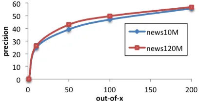
For an insight of the coverage for the entries deliv-ered by the DT graph, we extended the oot precision measure, to consider not only the first 10 entries, but the first X={1,10,50,100,200}entries (see Figure 2). Here we also show the coverage for different sized

Figure 2: Coverage on the LexSub test dataset for differ-ent DT graphs, usingout of Xentries.

datasets (10 and 120 million sentences). Amongst the 200 most similar words from the DT, a cover-age of up to 55.89 is reached. DT quality improves with corpus size, especially due to increased cover-age. This shows that there is considerable headroom for optimization for our contextualization method, but also shows that our automatic candidate expan-sions can provide a coverage that is competitive to lexical resources.

6 Conclusion

Additionally, we would like to adapt more advanced methods for the contextualization (Viterbi, 1967; Lafferty et al., 2001) that yield an all-words simulta-neous expansion over the whole sequence, and con-stitutes a probabilistic model of lexical expansion.

References

M. Baroni and A. Lenci. 2010. Distributional mem-ory: A general framework for corpus-based semantics.

Computational Linguistics, 36(4):673–721.

Chris Biemann and Martin Riedl. 2013. Text: Now in 2D! a framework for lexical expansion with contextual similarity. Journal of Language Modelling, 1(1):55– 95.

D. M. Blei, A. Y. Ng, and M. I. Jordan. 2003. Latent dirichlet allocation. J. Mach. Learn. Res., 3:993–1022. J. Boyd-Graber and D. M. Blei. 2008. Syntactic topic models. In Neural Information Processing Systems, Vancouver, BC, USA.

T. Van de Cruys, T. Poibeau, and A. Korhonen. 2013. A tensor-based factorization model of semantic compo-sitionality. InProc. NAACL-HLT 2013, Atlanta, USA. F. de Saussure. 1916. Cours de linguistique g´en´erale.

Payot, Paris, France.

J. Dean and S. Ghemawat. 2004. MapReduce: Simpli-fied Data Processing on Large Clusters. In Proc. of Operating Systems, Design & Implementation, pages 137–150, San Francisco, CA, USA.

S. Deerwester, S. T. Dumais, G. W. Furnas, T. K. Lan-dauer, and R. Harshman. 1990. Indexing by latent se-mantic analysis. Journal of the American Society for Information Science, 41(6):391–407.

S. Evert. 2004. The statistics of word cooccurrences: word pairs and collocations. Ph.D. thesis, IMS, Uni-versit¨at Stuttgart.

A. Goyal, J. Jagarlamudi, H. Daum´e, III, and T. Venkata-subramanian. 2010. Sketch techniques for scaling dis-tributional similarity to the web. InProc. of the 2010 Workshop on GEometrical Models of Nat. Lang. Se-mantics, pages 51–56, Uppsala, Sweden.

Z. S. Harris. 1951. Methods in Structural Linguistics. University of Chicago Press, Chicago, USA.

Thomas Hofmann. 1999. Probabilistic latent semantic indexing. In Proc. 22nd ACM SIGIR, pages 50–57, New York, NY, USA.

W. Kintsch. 2001. Predication. Cognitive Science, 25(2):173–202.

J. D. Lafferty, A. McCallum, and F. C. N. Pereira. 2001. Conditional random fields: Probabilistic models for segmenting and labeling sequence data. In Proc. of the 18th Int. Conf. on Machine Learning, ICML ’01, pages 282–289, San Francisco, CA, USA.

L. Lee. 1999. Measures of distributional similarity. In

Proc. of the 37th ACL, pages 25–32, College Park, MD, USA.

D. Lin. 1998. Automatic retrieval and clustering of similar words. InProc. COLING’98, pages 768–774, Montreal, Quebec, Canada.

M.-C. De Marneffe, B. Maccartney, and C. D. Man-ning. 2006. Generating typed dependency parses from phrase structure parses. InProc. of the Int. Conf. on Language Resources and Evaluation, Genova, Italy. D. McCarthy and R. Navigli. 2009. The english lexical

substitution task. Language Resources and Evalua-tion, 43(2):139–159.

G. A. Miller and W. G. Charles. 1991. Contextual corre-lates of semantic similarity. Language and Cognitive Processes, 6(1):1–28.

J. Mitchell and M. Lapata. 2008. Vector-based models of semantic composition. InProceedings of ACL-08: HLT, pages 236–244, Columbus, OH, USA.

R. Parker, D. Graff, J. Kong, K. Chen, and K. Maeda. 2011. English Gigaword Fifth Edition. Linguistic Data Consortium, Philadelphia, USA.

D. Pucci, M. Baroni, F. Cutugno, and R. Lenci. 2009. Unsupervised lexical substitution with a word space model. In Workshop Proc. of the 11th Conf. of the Italian Association for Artificial Intelligence, Reggio Emilia, Italy.

M. Richter, U. Quasthoff, E. Hallsteinsd´ottir, and C. Bie-mann. 2006. Exploiting the leipzig corpora collection. InProceesings of the IS-LTC 2006, Ljubljana, Slove-nia.

G. Ruge. 1992. Experiments on linguistically-based term associations.Information Processing & Manage-ment, 28(3):317 – 332.

P. Rychl´y and A. Kilgarriff. 2007. An efficient algo-rithm for building a distributional thesaurus (and other sketch engine developments). In Proc. 45th ACL, pages 41–44, Prague, Czech Republic.

Hinrich Sch¨utze. 1993. Word space. InAdvances in Neural Information Processing Systems 5, pages 895– 902. Morgan Kaufmann.

Ming Tan, Wenli Zhou, Lei Zheng, and Shaojun Wang. 2012. A scalable distributed syntactic, semantic, and lexical language model. Computational Linguistics, 38(3):631–671.

P. D. Turney and P. Pantel. 2010. From frequency to meaning: vector space models of semantics. J. Artif. Int. Res., 37(1):141–188.

A. J. Viterbi. 1967. Error bounds for convolutional codes and an asymptotically optimum decoding algorithm.