1
Sensitivity Analysis
on Service-Driven Network Planning
Paolo Di Francesco
Member, IEEE,
Jacek Kibiłda
Member, IEEE,
Francesco Malandrino,
Member, IEEE,
Nicholas Kaminski,
Member, IEEE,
Luiz A. DaSilva,
Fellow, IEEE
Abstract—Service providers are expected to play an increasingly central role in the mobile market and their relationship with the traditional mobile network operators (MNOs) is starting to change. The dilemma faced by over-the-top service-providers (OTT) is now whether to enter into a service level agreement with the MNOs (in the same spirit of mobile virtual network operator agreements) or to invest in deploying their own network infrastructure to serve their demand. The purpose of this paper is to study the factors shaping the agreements between OTTs and MNOs and how these factors impact network planning decisions. To this end, we build a synthetic model of cellular network deployment that explores how traditional mobile operators and OTTs compete in deploying new infrastructure. Using our model in conjunction with real-world data, we find that service-driven networks are heavily influenced by regulatory
decisions, and that cost structures and demand characteristics play non-marginal roles in the definition of service-driven networks.
Index Terms—Network Planning, SLA, Sensitivity Analysis, Optimization.
✦
1
I
NTRODUCTIONT
HE mobile market is rapidly changing and becoming more complex. Nowadays mobile network operators’ (MNOs) ability to generate revenue relies, firstly, on their subscribers and, secondly, on wholesale agreements with mobile virtual network operators (MVNOs) in a second-tier market [1]. Unfortunately this revenue model does not seem sustainable as the growing demand for capacity and data-rates forces MNOs to heavily invest in costly network infrastructure expansions and upgrades, impacting the prof-itability of running a mobile network. As a result, MNOs are showing interest in different business models [2].Meanwhile, many over-the-top service providers (OTTs) have based their success on the users’ perception oflimitless traffic [3] and Internet’s ubiquitousaccess. Mobile capacity shortages, and subsequent service degradation, would affect OTTs’ ability to generate profit. In particular, the OTTs offering bandwidth-intensive services such as HD video streaming on-demand or online gaming, which require strict quality of service (QoS), are the most exposed. Essentially, these OTTs are presented with two (non-exclusive) strate-gies: (i) to acquire capacity on-demand from MNOs, and (ii) to deploy their own infrastructure. Indeed we are already starting to witness similar scenarios. For example, Google’s Project Fi [4] offers to its subscribers both Wi-Fi, as part of Google’s effort to deploy its own infrastructure, and LTE connection, as part of Google’s MVNO agreement with traditional MNOs (i.e., Sprint and T-Mobile in the US). Other examples also exist and include the FreeBasics initiative by Facebook [5] and the Twitter deals [6].
A third strategy exists and aims at acting on the traffic demand. In its simplest form, certain types of traffic are charged at higher rates or downright forbidden. We leave
• All authors are with CONNECT, Trinity College Dublin, Ireland. This publication has emanated from research supported in part by re-search grants from Science Foundation Ireland (SFI) under Grant Numbers 10/IN.1/I3007 and 13/RC/2077.
these issues out of the scope of our work, as (i) they are seldom seen in real-world mobile networks, with the partial exception of MNOs blocking peer-to-peer traffic, and (ii) they would conflict with the right here, right now spirit driving users and providers of mobile services.
In our model, OTTs can decide to enter into service level agreements (SLAs) with an MNO to get a certain QoS for their services. In exchange for a fee, the MNO will reserve enough capacity to satisfy the QoS expected. The OTTs would need to decide whether it is more cost effective to rely on SLAs with selected MNOs or to deploy their own network infrastructure. The MNOs, in turn, would factor SLAs with OTTs into their decision of whether and how to expand their networks. In other words, we will enter the age ofservice-driven network expansion, and, more forward-looking,service-driven networks.
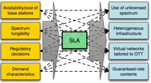
In order to study service-driven network expansion we need to assess, first, which factors are likely to influence SLAs, and second, the characteristics of the resulting net-works. The former are presented on the left hand side of Fig. 1 and include technical and non-technical aspects. Factors considered include the technologies available (e.g. LTE, WiFi) and their costs, public policy and regulation (e.g., whether to release new bands to the public, spectrum licensing schemes), and the characteristics of the demand. The resulting network characteristics are presented on the right hand side of Fig. 1 and include, for example, the level of heterogeneity of the resulting network in terms of both ownership and technology, the use of licensed/unlicensed spectrum, and the emergence of virtual networks tailored to OTTs. The likely result is a move from the current paradigm, where networks are designed, owned and controlled by MNOs, to a new one, where OTTs have a major role in the deployment of new infrastructure. Infrastructure will tend to become more heterogeneous, and integrate differ-ent equipmdiffer-ent, some of which will operate on unlicensed spectrum (e.g., ISM bands, as in LAA-LTE [7]).
Availability/cost of base stations
Spectrum fungibility
Regulatory decisions
Demand characteristics
Use of unlicensed spectrum
Heterogeneous infrastructure
Virtual networks tailored to OTT
Guaranteed-rate contents
[image:2.612.54.297.45.179.2]SLA
Fig. 1: The features of service-driven networks (blue boxes on the right hand side), and the factors driving them (yellow boxes on the left hand side) map into parameters and decision variables of our system model, respectively. Our high-level goal is to study the relationship between all those quantities, i.e., to untangle the network of arrows between the blocks.
and quantitatively, the impact of the different factors, listed on the left-hand side of Fig. 1, on the SLAs between an MNO and OTTs and on the planning decisions for service-driven networks. The first contribution of this work is a synthetic model of a cellular network deployment that accounts for some of the most relevant aspects of the service-driven network deployment described in Fig. 1 and how they interact with each other. For example, the set of tech-nologies available to OTTs in our model will depend on regulatory decisions, e.g., whether OTTs will be allowed to use licensed spectrum. Model parameters will account for the extent to which different parts of the spectrum can be considered equivalent to each other (e.g., intuitively, how many megahertz of Wi-Fi spectrum are needed to obtain the same performance of one megahertz of LTE spectrum), a concept often calledfungibility[8]. Our model captures the decisions made by OTTs about whether and how to deploy their own infrastructure; as an example, we have a decision variable expressing whether each operator deploys a base station of a certain type at a certain location, and parameters expressing the cost of doing so.
After presenting our model in Sec. 2, we detail in Sec. 3 our solution concept, showing how the main actors involved in the network expansion process efficiently make self-interested, near-optimal decisions. Sec. 4 contains estimates for all the factors we account for. Results, obtained for the real-world topology described in Sec. 5 and summarized in Sec. 6, show the impact of these factors on how and by whom service-driven networks will be built and operated.
2
S
YSTEM MODELIn this section, we present our system model, summarized in Fig. 2. We consider asnapshotof the network, taken during high-load conditions that are typically [9, Sec. 10.3.3.2] used as a reference when planning a network. The purpose of our model is to capture the network conditions in a challenging situation (as detailed in Sec. 4 and Sec. 5), so its infras-tructure can be planned accordingly. In this study, we also assume that backhaul is not a limiting factor for network capacity.
Technology Location User cluster Content
t∈ T l∈ Lt u∈ U c∈ C
Cost Demand
Capacity
p(l, t) τ(c, u)
k(l, t, u)
Deploy
yMNO(l, t), yOTT(l, t)∈ {0,1}
Serve
xMNO(c, l, t, u), xOTT(c, l, t, u)∈[0,1] Available
infrastructure
Demand characteristics Spectrum
fungibility
[image:2.612.313.561.46.214.2]Regulatory decisions
Fig. 2: Our system model. Grey, vertical blocks represent the model entities. Horizontal blocks correspond to parameters (green blocks) and decision variables (blue ones). Horizon-tal and vertical blocks cross when the parameter/variable represented by the horizontal block is indexed by the entity represented by the vertical one, e.g., a deployment decision is made for each technology and base station. Yellow clouds, corresponding to the boxes on the left hand side of Fig. 1, indicate the sources of our parameters.
The level of abstraction of our model is one of the most critical decisions we have to make. Cellular networks are highly complex entities, and any model trying to capture all this complexity would be exceedingly difficult to handle. As such, we employ simplified models to estimate, for example, the capacity for the different technologies, or the candidate locations of new base stations. However, it is important to stress that our goal is not to propose a comprehensive model for cellular network operations, but rather to study the relationships shown in Fig. 1 that influence network planning decisions ofservice-driven networks.
Another important decision deals with the level of de-terminism of our model. Three options were possible:
1) a fully probabilistic model, where we need to know the distribution for all quantities, and are able to estimate the distribution of the objective function and the probability that each constraint be met; 2) a hybrid model, where quantities are known as
distributions, but constraints need to be met with a static target probability;
3) a fully deterministic model, where parameters are known as fixed,worst-casevalues.
We opt for the third possibility, for simplicity and ef-ficiency considerations but most importantly because we are dealing with network planning decisions, which can take years to implement and whose effects can last for decades. These decisions are usually made based on long-term, worst-case projections and forecasts.
than they could, but this is consistent with the fact that no network provider is willing to risk service disruptions to their users [10].
System elements
Our system model includes four elements, represented by grey vertical blocks in Fig. 2: technologies, locations, user clusters and content types. The sets of technologies, loca-tions, clusters and content types are, within our system model, input data. In Sec. 4 and Sec. 5 we will discuss how and where this information is gathered.
Technologies t ∈ T represent the available types of net-work infrastructure. LTE macro and micro base stations as well as WiFi and mmWave access points correspond to different technologies; furthermore, base stations using different frequencies or power levels also correspond to different technologies. In general, if two infrastructure el-ements have different cost or coverage or performance, then in our model they correspond to different technologies. Some technologies require specific permissions or a license to operate (e.g. LTE base stations in licensed bands) and they are unlikely to be deployed by the OTTs. Therefore, we denote asTOTT ⊆ T the set of technologies available to
the OTTs, whileTMNO ≡ T corresponds to the technologies
available to the MNOs.
Locations l ∈ Lt represent the positions in space at which infrastructure of technology t ∈ T may be located. As an example, each building within an urban area may correspond to a location. In the following, we will often refer to the combination of a location l ∈ Ltand a base station typet∈ T as abase station.
User clusters u ∈ U represent groups of users that can be seen as co-located. Indeed, when performing network planning, we are not interested in the position or mobility of individual users, but rather in thetotalnumber of users in a constrained geographic area.
Last, Content typesc ∈ C(hereinafter “contents”) repre-sent the types of content users are interested in accessing such as HD video or on-line gaming.
Parameters
Parameters are known quantities associated with one or more elements of our system model. They are represented by green horizontal blocks in Fig. 2. From the viewpoint of our model, they are input values; however, as denoted by the yellow clouds in the figure, they actually come from the sources listed in Sec. 4.
The first parameter is theestimated capacityk(l, t, u)that a base station of technologyt∈ T, built in locationl ∈ Lt, would be able to offer to users in clusteru∈ U if it serves no other clusters, and it is based on a simplified model as expressed in:
k(l, t, u) =f(t)B(t)η(l, t, u), ∀t∈ T, l∈ Lt, u∈ U, (1)
where f(t)indicates the performance penalty incurred in when using unlicensed frequencies (see Sec. 4.2), B(t) is the bandwidth available to technology t(see Sec. 4.1), and
η(l, t, u) is the spectral efficiency that a base station of
technologytin locationlcan deliver to user clusteru. The
spectral efficiency is estimated using the Shannon bound and accounts for the distance between a location and a user cluster, the propagation model, and the specific technology employed. The maximum spectral efficiency achievable is also limited by the technology considered (see Sec. 4.1) as expressed in Eq. (2):
η(l, t, u)≤ηmax(t), ∀t∈ T, l∈ Lt, u∈ U. (2)
Notice that η-values can also account for site-specific information, if available – as an example, a site with a commanding view on top of a hill will have a higher efficiency than a tower on a flat ground surrounded by trees. Moreover, η-values also account for interference. Specifi-cally, interference from legacy, pre-existing deployments is embedded in the initial η-values, similarly to other site-specific information. Interference from new deployments, i.e., new base stations deployed by OTTs and MNOs, can be accounted for in a similar way, at the cost of recomputing theη-values, as discussed in Sec. 3.
We also need to know thecostp(l, t)of building a base station of technologyt ∈ T in locationl ∈ Lt. Cost ranges for different technologies can be extracted from the litera-ture, as detailed in Sec. 4. If such information is available, costs can also incorporate rent and maintenance, and site-specific features like existing rights-of-way to honor.
Costs p are per-year: they include recurring expenses (e.g., rent and energy) and the amortization of one-time costs, e.g., equipment. This allows our model to describe both green-field scenarios, where networks are built from scratch, and scenarios where network evolves from one gen-eration to the next. In the latter case, existing infrastructure is taken into account by lowering the cost of those (l, t)
combinations for which there is a base station of type t
already deployed at locationl.1
Last, we have thedemand τ(c, u)requested by users in clusteru∈ U for content typec∈ C. As discussed in Sec. 1, in our model the demand is a given parameter: MNOs and OTTs alike have no way of influencing it, neither through price incentives nor through traffic shaping techniques. As the authors of [11] put it, our users areimpatient.
Variables
Variables correspond to the decisions MNOs or OTTs make. They are represented by blue horizontal boxes in Fig. 2.
The first task the MNO faces is to propose an SLA fee to the OTTs, where the OTTs has to pay for their contents to be given a guaranteed bitrate. Such a fee may be a direct payment or some other form of revenue transfer from OTTs to the MNOs [?], [6]. In our model, we represent it through a per-megabitfee β charged to the OTT to have its traffic served by the MNO’s network.
The following decisions concern whether or not the OTTs deploya base station of technologyt∈ T at locationl∈ Lt represented through a binary variable yOTT(l, t). Parallel decisions are how to serve the users, i.e., the fraction of the total time and frequency resources (in LTE terminology, physical resource blocks, PRBs) a base station of technol-ogyt ∈ T, deployed at location l ∈ Lt, uses to meet the
demand of a subscriber requesting content c ∈ C located in clusteru ∈ U. This is expressed through a real-valued variable xOTT(c, l, t, u) ∈ [0,1]. Finally, the MNO has to deploy its own infrastructure and decide how to serve the residual demand for all the contents. These decisions can be represented by yMNO(l, t) andxMNO(c, l, t, u), respectively.
yMNOandxMNOindicate the same type of decision variables
asyOTTandxOTT, but they refer to the MNO rather than the
OTT.
3
S
OLUTION CONCEPTOur model accounts for the two main actors involved in deploying and managing service-driven networks, i.e., tra-ditional MNOs and OTTs. Each actor is self-interested and ultimately aims at maximizing its own profit. In this section, we detail the decision process they take part in, and how individual decisions are made.
3.1 Decision process
In our model, both OTTs and the MNO seek to maximize their profit (or, equivalently, minimize their costs, as revenue obtained from end users is assumed constant). Both need to decide what infrastructure of their own to deploy, in which location, and of what type. OTTs also need to decide how much to rely on the MNO to serve their content types, and the MNO needs to decide how much to charge OTTs to satisfy QoS requirements specified in the SLA for the OTTs’ contents.
In the first stage, the MNO decides the fee, i.e., the per-megabit price that OTTs have to pay if they want their contents to be delivered at a certain bitrate. Fees have an effect on the revenue the MNO collects. Intuitively, setting low fees indicates potentially low revenue for the MNO, which has to serve more traffic (hence update its network) for little additional revenue. On the other hand, setting very high fees represents a stronger incentive for OTTs to deploy their own infrastructure, rather than paying the MNO for their content to be delivered.
In the second stage, OTTs have to plan their infrastruc-ture. For each part of the topology, they can choose between having the MNO serve their demand therein – and paying the fee – or serving the demand themselves, deploying their own base stations – and bearing the related cost.
In the third stage, MNOs have to make decisions regard-ing deployment in their network. They know they have to serve all the demand left unserved by the OTTs in order to honor their commitments, by deploying the necessary infrastructure while minimizing their costs.
Note that, at every stage of the solution, we assume that the demandwillbe served, i.e., that the dimensioning problem is feasible. This assumption reflects the widespread belief that it will be possible for cellular networks to cope with the challenge posed by the increase in data demand, and we seek the best way to do so.
3.2 Individual steps
In the following, we detail how the MNOs and the OTTs make their decisions in each step of the process described in Fig. 4, and specifically, the problem they seek to optimize
and the method they employ to do it. We start by presenting the deployment decisions for each OTT, then the subsequent deployment decisions for the MNO. We reserve special attention to the problem of setting the fee at the end of this section.
OTT - minimize the costs to serve the demand
We now focus on the deployment decision problem from the point of view of the OTTs. We assume that each OTT knows the characteristics of its own demand, expressed as τ(ˆc, u), where ˆc is the content type that belongs to the OTT considered. The OTT can choose between serving the demand directly, deploying its own infrastructure, or using the MNO’s infrastructure and paying the feeβ. We assume that the β fee at this stage is known. Each OTT wants to maximize its profit, which is in this case equivalent to minimizing the total cost, i.e.,
min xOTT,yOTT
βX
u∈U
¯
τ(ˆc, u) + X t∈TOTT
X
l∈Lt
yOTT(l, t)p(l, t)
! (3)
X
t∈TOTT
X
l∈Lt
xOTT(ˆc, l, t, u)k(l, t, u)≤τ(ˆc, u), ∀u∈ U (4)
X
u∈U
xOTT(ˆc, l, t, u)≤yOTT(l, t), ∀t∈ TOTT, l∈ Lt, (5)
where τ¯ is the residual demand, expressed as the dif-ference between the total demand and the demand that is served by the OTT’s base stations:
¯
τ(ˆc, u) =τ(ˆc, u)− X
t∈TOTT
X
l∈Lt
xOTT(ˆc, l, t, u)k(l, t, u). (6)
The first term in Eq. (3) represents the fees paid to the MNO to serve the residual demand. The second term is the cost incurred by the OTT to deploy its own infrastructure. The OTT has no constraints to serve all its demand itself as indicated in Eq. (4): any residual demand τ¯ will be served by the MNO, as described earlier, in exchange for a fee. Moreover, constraint Eq. (4) indicates that the OTT does not serve more traffic demand then it has to, thus it prevents the quantity τ¯(ˆc, u)from taking negative values. Eq. (5) ensures that we properly account for the maximum capacity of the base stations. If theyOTT-value is zero, Eq. (5)
indicates that the base station cannot serve any user at all. If it is one, it prevents base stations from serving more traffic than they can, i.e., more than their capacity. The OTT is concerned with minimizing its total cost expressed in Eq. (3); if building no base station at all serves such a purpose, there is nothing forcing OTTs to do otherwise.
It is worth observing that the residual demand τ¯ is a decision variable for the OTTs, and, after we obtain theτ¯for all the content typesc ∈ C, it becomes an input parameter in the MNO deployment problem we examine in the next section.
MNO - minimize the deployment costs
At this stage, the MNO obtains theresidualdemandτ¯(c, u)
for the fee β. The MNO has to deploy infrastructure, i.e., setting yMNO-values to one, in order to serve the residual
demand. It seeks to satisfy the demand with minimum costs:
min xMNO,yMNO
X
t∈TMNO
X
l∈Lt
yMNO(l, t)p(l, t). (7)
X
t∈TMNO
X
l∈Lt
xMNO(c, l, t, u)k(l, t, u)≥τ¯(c, u), ∀c∈ C, u∈ U
(8) X
u∈U
X
c∈C
xMNO(c, l, t, u)≤yMNO(l, t), ∀t∈ TMNO, l∈ Lt.
(9)
Eq. (7) has to satisfy the constraints on the traffic de-mand and on the capacity expressed by Eq. (8) and Eq. (9). The constraint expressed by Eq. (8) ensures that the MNO provides enough capacity for all user clusters u ∈ U and contentsc∈ Cthe MNO must serve, while the constraint in Eq. (9) ensures that we properly account for the maximum capacity of the base stations and that only active base stations are used.
We note that the fee β does not appear in the MNO deployment problem – as at this stage, the MNO has already established the fee, and has to serve all the demand the OTT decides to delegate to it.
MNO - maximize the revenue by setting the feeβ
Setting the fee is the most complex task. It is a decision made by the MNO that depends on the response of the OTTs. The objective of the MNO is maximizing its own profit as shown in the following formula:
max
β β
X
u∈U
X
c∈C
¯
τ(c, u)− X
t∈TMNO
X
l∈Lt
yMNO(l, t)p(l, t)
!
(10)
The objective function expressed in Eq. (10) is composed by two terms. The first indicates the revenue that the MNO collects by serving the residual demand for each content type that belongs to the OTTs. The second term is the cost incurred in by the MNO to deploy additional infrastructure to serve the residual demand. The residual demand appears twice in this optimization problem, explicitly in the objective function in the first term, and implicitly in the second term in the form of the constraint in Eq. (8).
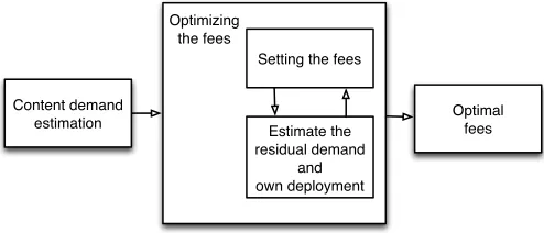
The residual demand ¯τ(c, u) depends upon decisions made by the OTTs that are affected by the feeβ, as we have seen previously. It is clear at this stage that the problem of optimizing the fees by the MNO is entwined with the problem faced by the OTTs to minimize their own costs. To circumvent this issue, we depict a strategy that we illustrate in Fig. 3.
At first, the MNO observes the traffic demand and infers the characteristics of the demand. The MNO then tries to optimize the fees by evaluating its utility function expressed in Eq. (10) for several values ofβand then selecting the best one. The MNO essentially has to solve a univariate discrete optimization problem that now involves an iterative pro-cess. The MNOestimatesthe residual demand left unserved
Content demand estimation
Setting the fees
Estimate the residual demand
and own deployment Optimizing
the fees
[image:5.612.314.561.45.151.2]Optimal fees
Fig. 3: Strategy to set the optimal fees from the MNO perspective. The MNO has to estimate the action of each OTT, assuming they seek to minimize their own cost.
by each OTT and subsequently the new infrastructure neces-sary to serve the whole residual demand for each value ofβ
by sequentially solving both the OTT’s deployment problem and its own.
Each fee’s configuration in fact yields a different residual demand ¯τ. However, the final network deployment corre-sponds to the one resulting from the optimumβ from the perspective of the MNO.
3.3 Solution strategy
In the following, we discuss how each of the problems presented above can be solved.
The OTTs and MNO deployments, corresponding to the internal boxes in Fig. 4, have the same structure. They are linear problems with integer (binary) and real variables, so they belong to the mixed integer linear programming (MILP) class; they can be solved to optimality with branch-and-cut algorithms using commercial state-of-the-art solvers such as Gurobi or CPLEX, provided that the size of the problem is not too large. If the size of the problem is too large, we would face the well-known scalability issues of MILP problems. In this case, we would turn to heuristic solutions such as the ones described in [12], originally for-mulated for set-covering problems. Their greedy approach has been shown, through extensive studies carried out on the OR problem library [13], to consistently perform close to the optimum, with a ratio between the solution they find and the optimal one being typically around1.2.
The problem solved by the MNO when setting the feeβ
is even more challenging, lacking a closed-form expression. However, in light of our strategy described in Fig. 3, the new problem becomes aunivariate problem in β, and therefore can be solved heuristically with root-finding algorithms such as the Brent method [14].
Root-finding algorithms explore several possible values of the decision variable, evaluate the value of the objective function, and use such information to select the next values to try. In our case, each iteration of the Brent method solves the problems Eq. (3) and Eq. (7) in sequence; their outputs are used to compute the payoff Eq. (10) and to find the optimal value ofβ.
therein.2Also notice that in practice, when deploying
addi-tional infrastructure, MNOs and OTTs can account for the resulting change in the interference environment through frequency planning and power control.
The scalability of the overall solution concept is ensured by the fact that the Brent method requires a limited number of iterations to converge, and each iteration takes a limited amount of time to solve subproblems Eq. (3) and Eq. (7).
Although they have been consistently observed to per-form very well in practice, neither the Brent method nor the heuristic in [12] come with a formal, absolute optimality guarantee. This is indeed consistent with our goals: we seek to confirm and uncover correlations between the conditions under which service-driven networks will operate and the features they will exhibit; to this end, heuristic solutions are essentially as useful as optimal ones.
Another relevant feature of our solution strategy is that it uses off-the-shelf components whenever available, either commercial solvers like CPLEX and Gurobi or well-established software like MATLAB and NumPy. Doing so allows us to focus on the solution strategy and the results it yields, as opposed to fine-tuning its building blocks. Furthermore, it provides us with the efficiency we need to process our datasets.
4
F
ACTORS SHAPING SERVICE-
DRIVEN MOBILENETWORKS
In this section, we describe the factors that will drive and shape service-driven mobile networks: the availability of new types of base stations; the fungibility of different por-tions of the spectrum; the regulatory decisions constraining the deployment of network infrastructure; the demand it will need to serve.
For each of these elements, we explain how it is captured within the model described in Sec. 2. We then review the es-timates for its value existing in the literature, and determine either a value or a range of values to use in our performance evaluation.
4.1 Base station technologies
Heterogeneity will be an important feature of service-driven mobile networks. Different types of base stations will coexist therein, including:
• LTE macro-base stations (macroBSs);
• LTE micro-base stations (microBSs); • millimeter-wave base stations (mmWave); • Wi-Fi access points.
Additional types of base stations can be added to T
as sufficiently detailed information about them becomes available such as Google’s Project Loon [15], LTE balloon-powered platforms operating in unlicensed bands used to provide LTE coverage to rural areas, or Facebook’s Connec-tivity Project [?].
Infrastructure types that operate in licensed bands (hence with exclusive usage rights) can only be deployed
2. Refreshing theη-values would marginally improve the accuracy of the results yielded by this model, at the cost of a substantially higher computational complexity. For this reason, we leaveη-values constant for our performance evaluation (Sec. 6).
by mobile network operators (e.g., LTE macroBSs and LTE microBSs at 1.8GHz and 2.6GHz), while technologies oper-ating in shared bands can be deployed by both MNO and OTT (e.g., mmWave, LTE microBSs at 3.5GHz, Wi-Fi) having different costs and fungibility (see Sec. 4.2).
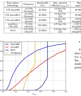
Tab. 1 summarizes the types of infrastructure we con-sider in this study, i.e., the elements of setT. For each of them, we indicate the frequency they operate at, their band-width, their maximum spectral efficiency, and the resulting maximum capacity – this is an upper bound on the values of parameterk(l, t, u). Notice that microBSs with exclusive and opportunistic access are considered as two separate elements ofT.
4.1.1 Cost
Estimating the cost of a base station is a difficult exercise. We gathered the figures indicated in Tab. 1 from peer-reviewed publications where available, and falling back to other sources such as business/technical reports when needed. Despite extensive research, we were unable to find a single cost estimate for mmWave base stations, other than generic claims that they will be inexpensive. We conjecture that their cost will lie between the most expensive Wi-Fi access points and the cheapest microBSs.
Recall that, as mentioned in Sec. 2, our costsp(l, t)are per-year. It follows that the values in Tab. 1 include both one-time costs (e.g., infrastructure) and recurring costs (e.g., energy or rent). Also, note that, for simplicity, we assume the price for each base station of technologyt∈ T to be the same regardless of the locationl∈ Lt.
4.1.2 Performance
Our system model (Sec. 2) includes a parameterη(l, t, u)≤ ηmax(t)describing the actual spectral efficiency attained by a base station of technology tdeployed at locationl when serving users in clusteru. The main factors influencingη -values are path-loss and interference, which we estimate through ITU- and 3GPP-vetted propagation models [22], [23].
Fig. 5 shows the distribution of the ηη(l,t,u)
max(t) ratio for
the different technologies, throughout all the experiments we run in our analysis. We can observe that technologies operating on licensed frequencies, e.g., macroBSs, tend to have a better ratio – even though the median macroBS has a spectral efficiency that barely exceeds 2 bps/Hz. mmWave and Wi-Fi never go beyond 50% and 70% of their potential efficiency.
4.2 Spectrum fungibility
IN
PU
T
P
AR
AMET
ER
S
Brent method
O
U
T
PU
T
(O
T
T
a
n
d
MN
O
D
EPL
O
YMEN
T
S)
select
β
OTT deployment
(MILP)
branch-and-cut or root finding
heuristics
MNO deployment
(MILP)
branch-and-cut or root finding
heuristics
Converge
? β
*
[image:7.612.128.487.45.164.2]=β
[image:7.612.69.333.207.519.2]Fig. 4: Solution strategy implementation overview.
TABLE 1: Infrastructure types populating setT.
Base station Frequency Bandwidth Max. spectral Max. Tx power Cost range Approx.
technology B(t) efficiencyηmax(t) capacity range
LTE macroBS (licensed)1.8 GHz 20 MHz 4.4 bps/Hz[16] 88 Mbps 40 dBm e[10000,60000]/year [17], [18] Several hundredsof meters
LTE microBS-L (licensed)2.6 GHz 20 MHz 4.4 bps/Hz[16] 88 Mbps 33 dBm e/year [17], [18][2000,10000] Few hundredsof meters
LTE microBS-S 3.5 GHz(shared) 20 MHz 4.4 bps/Hz[16] (fungibility<88 Mbps 33 dBm [2000,10000] Few hundreds
<1) e/year [17], [18] of meters
mmWave 73 GHz 500 MHz 2.25 bps/Hz <1125 Mbps 30 dBm [1000,2000] Tens of
[19], [20] (shared) (fungibility<1) e/year meters
Wi-Fi 2.4,5 GHz(shared) 20 MHz 3.12 bps/Hz[21] (fungibility<62.4 Mbps 24 dBm 1000 Tens of
<1) e/year [17], [18] meters
0.0 0.2 0.4 0.6 0.8 1.0
η/ηmax
0.0 0.2 0.4 0.6 0.8 1.0
CDF
macroBS
microBS
Wi-Fi
mmWaves
Fig. 5: Distribution of the ratio between the actual spectral efficiency values η(l, t, u) and the corresponding upper-boundsηmax(t), for different technologies.
As spectrum usage becomes more fluid, the concept of fungibility of spectrum becomes increasingly important [8]. Network operators have the ability to divert traffic between a number of different bands and technologies, buying this capacity on demand; fungibility provides an important tool to assess the relative usefulness of these options based on the goals of the operator.
Different portions of spectrum are not fungible, for three reasons:
• different frequencies are associated with different
bitrate and coverage;
• different frequencies typically require different
hard-ware running different protocols;
• unlicensed frequency bands are more prone to
con-gestion and interference than licensed ones.
[image:7.612.344.531.457.518.2]From the point of view of our model, all three aspects above are embedded in the fungibility parameterf(t)which we use to estimate the capacity k(l, t, u), as discussed in Sec. 4.1. Fungibility is a coefficient by which we further multiply the capacity as listed in Tab. 1; its values are presented in Tab. 2.
TABLE 2: Fungibility coefficients.
Technology Fungibilityrangef(t) Source
Small cells .
6−.9 [24] (WiFi and mmWave)
MicroBSs .
5−.75 [25] (in shared bands)
4.3 Regulatory decisions
Licensed spectrum is a scarce resource. Hence, who will be allowed to use it, and how, have a critical impact on network performance, and heavily depend on regulatory decisions. In our work, we examine two scenarios concerning which portions of the spectrum, and under which conditions, OTTs have access to:
• LTE-standard complying base stations can only
transmit in licensed spectrum. OTTs cannot operate microBSs in shared bands [Scenario A].
• LTE-standard complying base stations can be
de-ployed in both licensed and shared spectrum. The OTT and MNO can deploy microBSs, but in shared bands they experience a fungibility coefficient lower than one, as reported in Tab. 2 [Scenario B].
Selecting one or the other of these scenarios changes the elements of setTOTT, as well as the adjusted capacity kof
4.4 Demand
The total demand and set C of content types depend on the reference scenario we consider, as discussed later in Sec. 5. We seek to study the impact that spatial clustering of intensities for a particular content, i.e., whether users requesting a particular content tend to be close to each other or not, has on service-driven networks. We quantify this clustering through the Hegyi index [26], used to express the clustering strength between spatially distributed points (user clusters, in our case) associated to a continuous value (contents, in our case). The Hegyi index for user clusteru
and contentcis:
H(c, u) = N
X
i=1
τ(c, u)
τ(c, u)(1 +||u+ni(u)||)
, (11)
where||·||denotes the Euclidean distance between two user clusters,ni(u)denotes thei-th closest cluster tou, andN is a parameter denoting the number of nearest user clusters we account for (in our case,N = 5). The complementarity value associated with a specific content typec′ ∈ C
is defined as the average over all user clustersu∈ U ofH(c′
, u):
H(c′) = 1
|U|
X
u∈U
H(c′, u). (12)
The complementarity value defined in Eq. (12) ulti-mately tells us how spatially-clustered the demand for a certain content type tends to be. Intuitively, we can expect that a more clustered demand is easier to serve through such targeted infrastructure as the one that can be deployed by OTTs. Location-specific services, e.g., tourist informa-tion [27] or advertisements for local businesses [28], are often mentioned as prime examples of content associated to high complementarity values. Other such contents include maps, especially for mobile and vehicular users [29], and, more recently, augmented-reality games such as Pokemon Go [30].
We investigate the correlation between the complemen-tarity of the demand for a particular content with the traits of the resulting network in Sec. 6. Notice that we do notassumea certain complementarity value for our study; rather, we explore what happens if high-complementarity, location-based services come to pass.
5
R
EFERENCE SCENARIOIn this section, we describe the reference scenario we employ for our simulations, i.e., how we populate the sets of user clustersU and (potential) base station locationsLtfor each technologyt ∈ T, and how we set the demandτ(c, u)for each user cluster and content type.
User clusters and locations: our reference topology is the entire urban area of Dublin, Ireland, as indicated by the Central Statistics Office (CSO) Ireland in [31]. We place a total of2,210user clusters throughout this area, such that each cluster represents a population of at most 300 people. It follows that more populated areas tend to have more user clusters; this enables us to study dense deployments in such areas while keeping the overall complexity low. We also assume that the LTE macroBSs deployment is already in place to ensure full coverage and mobility and it is given
by the available on-line data [32]. In fact, it makes sense for the MNOs to consider in network planning problems the infrastructure already deployed, especially the costly one.
The possible locations in Lt for technology t ∈ T are placed on a regular grid with the inter-site distance depending on the coverage range. For example, the inter-site distance for LTE microBS is 100 meters, while for WiFi and mmWave is 50 meters.
Service providers demand and initial deployment:
setting the demand values τ(c, u) is a complex task, for which little information is available and some speculation is unavoidable. We proceed as follows:
1) we set the total demand for each user clusteru, i.e., P
c∈C τ(c, u);
2) we decide how this total demand is split between contents;
3) we adjust the resulting demand complementarity.
We accomplish the first step by leveraging a set of real-world call-detail record (CDR) information from an Irish mobile operator, referring to a period of two weeks in 2013. We then augment that total demand according to the projections of the Cisco Virtual Network Index [33], and obtain an estimate for mobile data demand over the next 5 years.
Breaking down such an aggregated demand into indi-vidual demand for each content is another complex prob-lem. We turn to the measurement work [34], which identifies fourtraffic patterns, i.e., sets of content types, that users in each location were found to conform to. We assume then that a particular content type can be associated with an OTT. We randomly associate one traffic profile to each user cluster, adjusting the average distance between two user clusters belonging to the same profile. Intuitively, a small distance means that users wanting the same content types tend to be located close together, hence a higher comple-mentarity as defined in Eq. (12).
Finally, we select the most popular of contents types ascˆ∈ C, i.e., the demand volume that the OTT has to serve (either through the MNO’s network or its own). All other content types are assumed to belong to the MNO.
6
R
ESULTSIn this section we analyze the relationship between the parameters of our model and the resulting base station deployments. Intuitively, we try different combinations of input parameters (the yellow boxes in Fig. 1, e.g., different levels of cost for macroBSs), and observe how andhow much they impact the resulting network deployment (the blue boxes in Fig. 1, e.g., how many base stations are deployed and by whom).
As summarized in Fig. 6, we split our analysis into two parts. First, in Sec. 6.1, we seek to understand which input parameters have the deepest influence on the fee β⋆ that the MNO will charge to the OTT for using its network; then, in Sec. 6.2, we assess howβ⋆ influences the network deployment.
IN
PU
T
P
AR
AMET
ER
S
Brent method
OTT deployment
(MILP)
branch-and-cut or root finding
heuristics
MNO deployment
(MILP)
branch-and-cut or root finding
heuristics
β
*(a)
IN
PU
T
P
AR
AMET
ER
S ,
deployment (MILP)
branch-and-cut or root finding
heuristics
MNO deployment
(MILP)
branch-and-cut or root finding
heuristics
β
*O
U
T
PU
T
(O
T
T
a
n
d
MN
O
d
e
p
lo
yme
n
t)
[image:9.612.111.505.46.167.2](b)
Fig. 6: Analysis methodology. Once the process in Fig. 4 is completed, we analyse the impact of the input parameters by looking at the problem from two different angles. In (a), we check the influence of the input parameters on the price imposed by the MNO on the OTT (β⋆). In (b), we seek to find out the influence of the same input parameters and theβ⋆ (now considered as an input parameter) on the output deployment.
L M H
β⋆ 0%
20% 40% 60% 80% 100%
Fr
eq
ue
nc
y
of
β
⋆ v
al
ue
s Scenario AScenario B
(a)
L M H
β⋆ 0%
20% 40% 60% 80% 100%
Fr
eq
ue
nc
y
of
β
⋆ v
al
ue
s Scenario AScenario B
(b)
L M H
β⋆ 0%
20% 40% 60% 80% 100%
Fr
eq
ue
nc
y
of
β
⋆ v
al
ue
s Scenario AScenario B
(c)
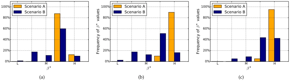
Fig. 7: Distribution of the feeβ⋆for low (a), medium (b), high (c) complementarity. Bars represent the fraction ofβ⋆values that are low, medium, high.
network of relationships shown in Fig. 1 and study, in its stead, only those involvingβ⋆itself.
6.1 What determinesβ⋆?
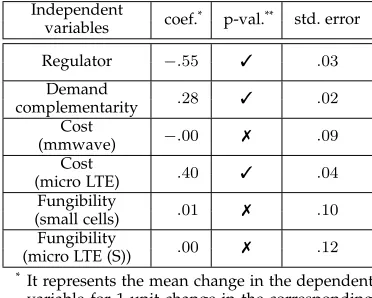
The first part of the analysis, as indicated in Fig. 6(a), seeks to assess the key determinants on the variations of β⋆. We carry out a sensitivity analysis employing a multivariable ordinary least-squared (OLS) regression model, where the independent variables are all the ones on the left hand side of Fig. 1 and the dependent variable isβ⋆. The total number of parameter combinations we study is 720.
The results of the regression model are summarized in Tab. 3. As per Fig. 6(a), in this part of our analysis β⋆ is the dependent variable and all other quantities – regula-tor decisions, demand complementarity, costs, fungibility values – are independent variables. We can immediately notice that among the input parameters chosen to analyse
β⋆, only three are actually statistically significant at a p-value of .01. First, both the regulator and the cost of LTE microBSs have a negative impact on the fee charged by the MNO. The (binary)3 variable modelling the regulator
allows the OTT access to deploy LTE microBSs in shared spectrum. Infrastructures with wider coverage appear to be very appealing to OTTs since they allow the OTTs to
3. We remark that, while OLS analysis for generic categorical vari-ables requires such special techniques as dummy varivari-ables or one-hot encoding, binary independent variables can be used as they are.
serve lower-demand subscribers with less infrastructure. As a consequence, the MNO tries to discourage the OTT from deploying many LTE microBS by setting a lower price on the OTT traffic it can serve. Second, the demand complemen-tarity has a non-obvious positive impact on theβ⋆. When the majority of the demand is clustered, it can be served with fewer base stations. As a result, the MNO’s best action is to set a high fee so as to ensure some gain at least in those regions where the OTT does not find it convenient to deploy any infrastructure. This dual effect is also captured by the histograms in Fig. 7. Preventing OTTs from deploying microBSs, i.e., moving from scenario B to scenario A as defined in Sec. 4.3, generally yields fewer values in the lower bins and more in the higher ones, i.e., increasing the fee – intuitively, reducing the freedom of action of OTTs increases the fee they are required to pay.
For completeness, we also report in Tab. 3 the coefficient of determination, R2. It measures how well the model captures the variation of the dependent variable [35] and it is defined as:
R2= 1−
P
i(si−s¯)
2
P
i(si−fi)2
, (13)
[image:9.612.66.553.230.367.2]TABLE 3: Standardized regression analysis coefficients, rel-ative to the first part of our analysis (Fig. 6(a)), where β⋆ is the dependent variable and the quantities listed in the first column are independent variables. The coefficent of determination isR2=.60. (see Fig. 6(a)).
Independent
coef.* p-val.** std. error
variables
Regulator −.55 ✓ .03
Demand .28 ✓ .02
complementarity
Cost −.00 ✗ .09
(mmwave)
Cost .40 ✓ .04
(micro LTE)
Fungibility .01 ✗ .10 (small cells)
Fungibility .00 ✗ .12 (micro LTE (S))
*It represents the mean change in the dependent
variable for 1 unit change in the corresponding independent variable while holding the other independent variables to their mean.
**✓ indicates statistical significance (p-value< .01) while✗indicates not statistically significant
(p-value> .01).
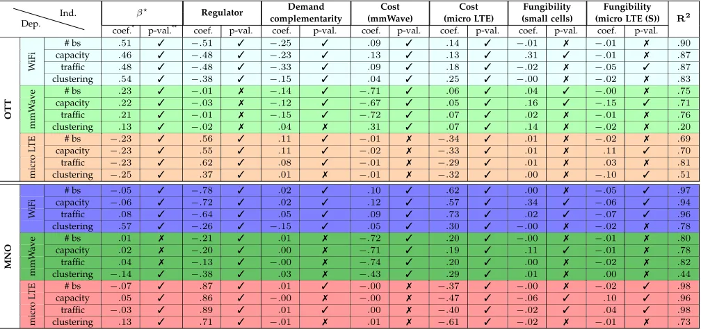
6.2 What influences the deployment?
In the second part of the analysis, we focus on the network deployment. We identify, for each operator (i.e., MNO and OTT) and each technology (e.g. WiFi, mmWave, and LTE micro BSs) three parameters of interest: amount of infras-tructure built, the capacity supplied and the traffic served by such infrastructure.
There are two main differences from the analysis in Sec. 6.1: first, theβ⋆identified in Sec. 6.1 takes now a much more important role. Together with the original input pa-rameters, we investigate the impact of theβ⋆variable on the deployment, in particular the decision the OTT of whether or not to deploy infrastructure to serve its own demand. To carry out this study we run multiple multivariable OLS regressions, focusing on one outcome variable at a time.
In Tab. 4 we summarize the results obtained by check-ing one dependent variable at a time. Tab. 4 should be read row-wise, where each row reports the coefficients and p-value of an individual multivariable regression model on the corresponding network deployment output. Tab. 4 lists network deployment quantities (i.e., number of base stations, capacity, traffic served, and level of clustering) grouped by operators and technology in the first column. Remaining columns represent independent variables (i.e.,
β⋆, regulatory decisions, demand characteristics, technolo-gies cost, fungibility), with the final column reporting the
R2value.
A few observations are noteworthy. First, only the cost for LTE microBSs is significant to all network planning actions. Second, the upper part of Tab. 4 reveals that, for the OTT, theβ⋆and the regulatory decisions are influential parameters. They affect all the deployment decisions taken by the OTT, and, to a different extent, the MNO, i.e., defining the heterogeneity of the number of base stations and capac-ity deployed. The demand complementarcapac-ity mainly impacts the planning decisions of the OTT, while the decisions taken by the MNO are mostly driven by infrastructure cost.
6.2.1 Infrastructure cost
As we have seen in Tab. 4, infrastructure cost has a sig-nificant influence on the deployment decisions made by operators and service providers. In Fig. 8(a) we show the number of base stations of each type deployed by the OTT and the MNO. On thex-axis is the cost (relative to the WiFi) to deploy and maintain a mmWave or an LTE microBS. OTTs are allowed to deploy LTE microBSs in opportunistic access spectrum, i.e., we are in scenario B as described in Sec. 4.3.
Let us compare the group of bars on the left hand side of Fig. 8(a), indicating low costs for infrastructure, with the group of bars in the middle and the right hand side of Fig. 8(a) indicating medium and high costs respectively: if infrastructure is sufficiently cheap, the best course of action for the MNO and OTT is to rely more on LTE microBSs, the ones that give the best compromise between coverage and capacity. As the infrastructure cost increases, both MNO and OTT rely more on WiFi infrastructure. Fig. 8(b) shows how the capacity evolves according to changes in the costs. High-capacity/short-range technologies will only be successful if their cost is low enough; otherwise, due to their low coverage range, they are unlikely to be deployed. Fig. 8(b) and Fig. 8(c) display an interesting effect: higher capacity does not necessarily translate into more traffic being served if the capacity is very localized, as it is the case with short-range infrastructure. In fact, as the cost of infrastructure increases, the OTT relies more on the MNO to serve its demand, as it again can be observed in Fig. 8(c).
Fig. 9 and Fig. 10 provide a closer look at how the combi-nation of prices for microBSs and mmWave influence the de-cisions made by the OTT and MNO. Fig. 9(a) and Fig. 10(a) show that OTTs essentially choose between microBSs and Wi-Fi access points, while they resort to mmWave base sta-tions only when their cost is low. Consistently with Fig. 8(b), Fig. 9(b) and Fig. 10(b) show that mmWave base stations skew the network capacity, even when, as we can see in Fig. 8(c), Fig. 9(c) and Fig. 10(c), microBSs serve most of the traffic.
Service-driven networks will be different from current ones in that the network technology providing the most capacity maynot be the one serving the most traffic. This leaves room for innovative applications e.g., proximity ser-vices and machine-to-machine systems – as long as they do not require ubiquitous, continuous coverage.
6.2.2 Demand complementarity
As seen in Sec. 6.1 and in particular in Fig. 7, the demand complementarity has a non-negligible impact on the feeβ⋆ that the MNO charges the OTT to carry its traffic, i.e. theβ
value that maximizes the quantity in Eq. (10).
TABLE 4: Standardized regression analysis coefficients, p-values and R2for the system in Fig. 6(b).
Dep.
Ind. β⋆
Regulator complementarityDemand (mmWave)Cost (micro LTE)Cost (small cells)Fungibility (micro LTE (S))Fungibility R2
coef.* p-val.** coef. p-val. coef. p-val. coef. p-val. coef. p-val. coef. p-val. coef. p-val.
# bs .51 ✓ −.51 ✓ −.25 ✓ .09 ✓ .14 ✓ −.01 ✗ −.01 ✗ .90
capacity .46 ✓ −.48 ✓ −.23 ✓ .13 ✓ .13 ✓ .31 ✓ −.01 ✗ .87
traffic .48 ✓ −.48 ✓ −.33 ✓ .09 ✓ .18 ✓ −.02 ✗ −.05 ✓ .87
W
iF
i
clustering .54 ✓ −.38 ✓ −.15 ✓ .04 ✓ .25 ✓ −.00 ✗ −.02 ✗ .83
# bs .23 ✓ −.01 ✗ −.14 ✓ −.71 ✓ .06 ✓ .04 ✓ −.00 ✗ .75
capacity .22 ✓ −.03 ✗ −.12 ✓ −.67 ✓ .05 ✓ .16 ✓ −.15 ✓ .71
traffic .21 ✓ −.01 ✗ −.15 ✓ −.72 ✓ .07 ✓ .02 ✗ −.01 ✗ .76
m
m
W
av
e
clustering .13 ✓ −.02 ✗ .04 ✗ .31 ✓ .07 ✓ .14 ✗ −.02 ✗ .20
# bs −.23 ✓ .56 ✓ .11 ✓ −.01 ✗ −.34 ✓ .01 ✗ −.02 ✗ .69
capacity −.23 ✓ .55 ✓ .11 ✓ −.02 ✗ −.33 ✓ .01 ✗ .11 ✓ .70
traffic −.23 ✓ .62 ✓ .08 ✓ −.01 ✗ −.29 ✓ .01 ✗ .03 ✗ .81
O
T
T
m
ic
ro
L
T
E
clustering −.25 ✓ .37 ✓ .01 ✗ −.01 ✗ −.32 ✓ .00 ✗ −.10 ✓ .51
# bs −.05 ✓ −.78 ✓ .02 ✓ .10 ✓ .62 ✓ .00 ✗ −.05 ✓ .97
capacity −.06 ✓ −.72 ✓ .02 ✓ .12 ✓ .57 ✓ .34 ✓ −.06 ✓ .94
traffic .08 ✓ −.64 ✓ .05 ✓ .09 ✓ .73 ✓ .02 ✓ −.07 ✓ .96
W
iF
i
clustering .57 ✓ −.26 ✓ −.15 ✓ .05 ✓ .30 ✓ −.00 ✗ −.02 ✗ .78
# bs .01 ✗ −.21 ✓ .01 ✗ −.72 ✓ .20 ✓ −.00 ✗ −.01 ✗ .80
capacity .02 ✗ −.20 ✓ .00 ✗ −.71 ✓ .19 ✓ .11 ✓ −.01 ✗ .78
traffic .04 ✗ −.13 ✓ −.00 ✗ −.74 ✓ .20 ✓ .00 ✗ −.02 ✗ .82
m
m
W
av
e
clustering −.14 ✓ −.38 ✓ .03 ✗ −.43 ✓ .29 ✓ .01 ✗ .00 ✗ .44
# bs −.07 ✓ .87 ✓ .01 ✓ −.00 ✗ −.37 ✓ −.00 ✗ −.02 ✓ .98
capacity .05 ✓ .86 ✓ −.00 ✗ −.00 ✗ −.47 ✓ −.06 ✓ .10 ✓ .96
traffic −.03 ✓ .89 ✓ .01 ✓ .00 ✗ −.40 ✓ −.02 ✓ .04 ✓ .98
M
N
O
m
ic
ro
L
T
E
clustering .13 ✓ .71 ✓ −.01 ✗ .01 ✗ −.61 ✓ −.02 ✗ −.01 ✗ .73
*It represents the mean change in the dependent variable for 1 unit of change in the corresponding independent variable while holding the others. **✓indicates statistical significance (p-value< .01) while✗indicates not statistically significant (p-value> .01).
***We omit the standard error and the 95% confidence interval in order to keep the table more readable. ****The colors are consistent with Fig. 8, Fig. 9, and Fig. 10 in order to help the reader to follow the discussion.
LL MM HH
Infrastructure costs
0 100 200 300 400 500
#
ba
se
st
ati
on
s
MNO Wi-Fi MNO mmWave MNO microBSs (L+S)
OTT Wi-Fi OTT mmWaves OTT microBSs (S)
(a)
LL MM HH
Infrastructure costs
0 5 10 15 20 25
Ca
pa
city
[G
bit/se
c]
MNO Wi-Fi MNO mmWave MNO microBSs (L+S)
OTT Wi-Fi OTT mmWaves OTT microBSs (S)
(b)
LL MM HH
Infrastructure costs
0 1 2 3 4 5
Tra
ffic
se
rve
d [
Gb
it/se
c]
MNO Wi-Fi MNO mmWave MNO microBSs (L+S)
OTT Wi-Fi OTT mmWaves OTT microBSs (S)
[image:11.612.57.555.321.481.2](c)
Fig. 8: Number of base stations deployed (a), capacity supplied (b), traffic served (c) for different combinations of prices. The error bars indicate the 95% confidence interval.
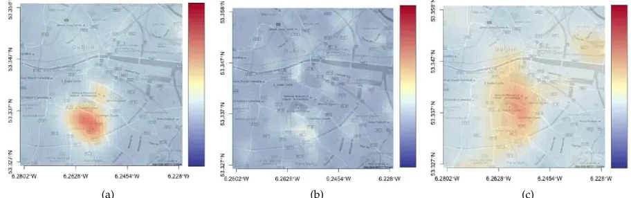
demand of contentˆc. Instead the capacity deployed in the reference scenario complements the one deployed by the MNO rather than overlapping with it.
When we lower the complementarity to its minimum value, in Fig. 12, an entirely different picture emerges. The demand for contentˆc(Fig. 12(a)) is distributed over a wider area, mostly in the South. As we can see from Fig. 12(b), the OTT deploys a much lower number of base stations, in lo-cations throughout the topology. Also notice from Fig. 12(c) how some of the demand for contentˆcis also served by the MNO.
In summary, Fig. 11 and Fig. 12, obtained for different values of complementarity, show two very different net-works. In Fig. 11, OTT and MNO complement each other in serving the traffic demand; in Fig. 12 the MNO builds a high-capacity network with vast coverage and the OTT pays a (moderate) fee to use it.
7
R
ELATED WORKA first body of works our paper relates to deals with the planning of mobile networks. Particular emphasis is put on their different conditions and requirements with respect to traditional LTE networks, including radically different outdoor and indoor scenarios [36], ultra-dense de-ployments [37], and device-to-device communications [38].
peer-Cost mmWave L
M
H Cost mic roBs
L M H
#
Base stati ons
0 100 200 300 400 MNO mmWave
MNO Wi-Fi MNO microBSs (L+S)
(a)
Cost mmWave L
M
H Cost mic roBs
L M H
Capa city [Gb it/se
c]
0 10 20 30 MNO mmWave
MNO Wi-Fi MNO microBSs (L+S)
(b)
Cost mmWave L
M
H Cost mic roBs
L M H
Traffic serve d [Gb it/se
c]
0 1 2 3 4 MNO mmWave
MNO Wi-Fi MNO microBSs (L+S)
[image:12.612.69.553.46.184.2](c)
Fig. 9: MNO. Number of base stations deployed (a), capacity supplied (b), traffic served (c) for all costs combinations.
Cost mmWave L
M
H Cost mic
roBs
L M H
#
Base statio
ns
0 100 200 300 400 OTT mmWave
OTT Wi-Fi OTT microBSs (S)
(a)
Cost mmWave L
M
H Cost mic
roBs
L M H
Capa city [ Gbit/se
c]
0 10 20 30 OTT mmWave
OTT Wi-Fi OTT microBSs (S)
(b)
Cost mmWave L
M
H Cost mic
roBs
L M H
Traffic serve d [Gb it/se
c]
0 1 2 3 4 OTT mmWave
OTT Wi-Fi OTT microBSs (S)
[image:12.612.61.553.216.351.2](c)
Fig. 10: OTT. Number of base stations deployed (a), capacity supplied (b), traffic served (c) for all costs combinations.
(a) (b) (c)
Fig. 11: High complementarity: location of the demand for content typecˆ(a); capacity deployed by the OTT (b) and the MNO (c).
(a) (b) (c)
[image:12.612.73.529.381.526.2] [image:12.612.74.530.574.717.2]reviewed literature.
Fungibility studies are also very relevant to our work. Examples include [8], which introduced several methods to compute fungibility scores, and [40], where those scores are refined. A set of related works aims at the more general objective of assigning a value to wireless spectrum, for the purpose of introducing fluid networks [41], and enabling spectrum trading [42], [43]. The ultimate purpose is evalu-ating the effectiveness of dynamic spectrum use, where [44] specifically accounts for regulatory decisions.
Finally, our work is related to such real-world mea-surements of data demand as [34], [45], [46]. Two of these reports show that different types of data demand tend to be spatially correlated [45], [46]. These studies were concerned with web services and smartphone apps only; however, similar conclusions were drawn when more general mobile demand was considered, as in [34], where the authors operated on flow-level information sent to and from cellular devices. Their study reveals that various data applications are not equally popular across all cells, and that “the pop-ularity of some applications is more skewed than others across cells”. Moreover, a few applications dominate others given their relative traffic volume, and applications can be grouped into traffic profiles that describe application usage distribution for any given cell. Other works, e.g., [47], [48] have studied real-world deployments of cellular networks, and found that some spacial features thereof are remarkably similar throughout mobile operators and cities.
8
C
ONCLUSIONThis paper sought to study the mobile network expansion driven by the OTT’s service needs and to assess, first, the factors that are likely to impact deployment decisions by OTTs and MNOs, and second, the characteristics of the resulting networks.
We found that the factors with the deepest influence on the final network are not technical but rather economic (e.g., the cost of base stations) and regulatory (e.g., the type of spectrum and technologies OTTs are allowed to use). Different combinations of these factors yield radically different networks: in some cases, OTTs and MNOs deploy separate networks that complement each other; in others, MNOs find it convenient to offer plentiful, cheap capacity to OTTs, which have no incentive to deploy their own networks. Furthermore, the technologies providing most of the network capacity (most notably, mmWave) will not serve most of the traffic, leaving plenty of opportunities for innovative applications such as proximity services and M2M.
Real-world datasets such as ours are difficult to come by, and one might wonder how general our conclusions based on Dublin city are. While a definite answer would require more datasets, the authors of [48] found that base station deployments of different operators in different cities have remarkably similar spatial properties and can be modeled with very similar statistic models. This, along with the fact that we study different demand profiles with different complementarity values, affords to our study a high level of generality. Indeed, our conclusions about the importance of MNO fees are consistent with the findings of [49], which
uses stochastic distributions for both demand and infras-tructure.
R
EFERENCES[1] R. Xia et al., “Business Models in the Mobile Ecosystem,” in Conference on Mobile Business and Global Mobility Roundtable, 2010. [2] Value Partners, “Mobile 2015: New Spectrum,
Dif-ferent Business Models, More Competition?” [Online]. Available: http://www.valuepartners.com/downloads/PDF Comunicati/value-partners-120210-mobile-2015-henry-alty.pdf [3] T. Giles et al., “Cost Drivers and Deployment Scenarios for
Fu-ture Broadband Wireless Networks - Key Research Problems and Directions for Research,” inIEEE Vehicular Technology Conference Spring, 2004.
[4] Project Fi – Google. [Online]. Available: https://fi.google.com/ [5] Facebook Inc. [Online]. Available: https://info.internet.org/en/
story/free-basics-from-internet-org/
[6] S. Datoo, “Twitter’s latest deal points to ambitions in emerging markets,”The Guardian, 2013.
[7] H. Zhanget al., “Coexistence of Wi-Fi and Heterogeneous Small Cell Networks Sharing Unlicensed Spectrum,”IEEE Communica-tions Magazine, 2014.
[8] M. Weisset al., “When is Electromagnetic Spectrum Fungible?” in IEEE New Frontiers in Dynamic Spectrum Access Networks, 2012. [9] M. Nawrockiet al.,Understanding UMTS Radio Network Modelling,
Planning and Automated Optimisation: Theory and Practice. John Wiley & Sons, 2006.
[10] Credit Suisse, “U.S. Wireless Networks Running at 80% of Capacity,” 2011. [Online]. Available: http://benton.org/node/ 81874
[11] Y. J. Chianget al., “Performance and Cost-Effectiveness Analyses for Cloud Services Based on Rejected and Impatient Users,”IEEE Transactions on Services Computing, vol. 9, no. 3, pp. 446–455, 2016. [12] A. Caprara et al., “Algorithms for the set Covering Problem,” Annals of Operations Research, vol. 98, no. 1-4, pp. 353–371, 2000. [13] F. C. Gomes et al., “Experimental Analysis of Approximation
Algorithms for the Vertex Cover and Set Covering Problems,” Computers & Operations Research, vol. 33, no. 12, pp. 3520–3534, 2006.
[14] R. P. Brent,Algorithms for minimization without derivatives. Engle-wood Cliffs, N.J: Prentice-Hall, 1972.
[15] Google Inc. [Online]. Available: http://www.google.com/loon/ [16] “LTE Technical Modelling Revised Methodology,”
OFCOM White Paper, 2012. [Online]. Avail-able: http://stakeholders.ofcom.org.uk/binaries/consultations/ award-800mhz/annexes/annex14.pdf
[17] M. Paolini, “The Economics of Small Cells and Wi-Fi offload,” Senza Fili Consulting, Tech. Rep., 2012.
[18] E. Hossain, “Evolution Toward 5G Cellular Networks: A Radio Resource and Interference Managment Perspective,” inIEEE In-ternational Conference on Communications (ICC) Tutorials, 2014. [19] S. Ranganet al., “Millimiter Wave Cellular Wireless Networks:
Potentials and Challenges,”Proceedings of the IEEE, 2014. [20] T. S. Rappaport et al., “Millimeter-Wave Urban Channels
Com-munications: Channel Models, Capacity Limits, Challenges and Opportunities,”IEEE Communications Theory Workshop, 2014. [21] E. Perahia and R. Stacey,Next generation wireless LANs : 802.11n
and 802.11ac. Cambridge University Press, 2013.
[22] 3GPP Technical Report 36.814, “Further Advancements for E-UTRA Physical Layer Aspects,” 2010.
[23] ITU. Recommendation ITU-R P.1411-1. https://www.itu.int/ dms pubrec/itu-r/rec/p/R-REC-P.1411-1-200102-S!!PDF-E.pdf. [24] K. Lee et al., “Mobile Data Offloading: How Much Can Wi-Fi
Deliver?”Networking, IEEE/ACM Transactions on, vol. 21, no. 2, pp. 536–550, 2013.
[25] I. Macalusoet al., “Complexity of Spectrum Activity and Benefits of Reinforcement Learning for Dynamic Channel Selection,” Se-lected Areas in Communications, IEEE Journal on, vol. 31, no. 11, pp. 2237–2248, 2013.
[26] J. Illian et al., Statistical Analysis and Modelling of Spatial Point Patterns (Statistics in Practice), 1st ed. Wiley-Interscience, 2008. [27] N. Aloket al., “AdTorrent: Digital Billboards for Vehicular