Munich Personal RePEc Archive
Multivariate bubbles and antibubbles
Fry, John
University of Sheffield
19 May 2014
Online at
https://mpra.ub.uni-muenchen.de/56081/
Multivariate bubbles and antibubbles
John Fry∗
May 2014
Abstract
In this paper we develop models for multivariate financial bubbles and antibubbles based on statistical physics. In particular, we extend a rich set of univariate models to higher dimensions. Changes in market regime can be explicitly shown to represent a phase transition from random to deterministic behaviour in prices. Moreover, our multivariate models are able to capture some of the contagious effects that occur during such episodes. We are able to show that declining lending quality helped fuel a bubble in the US stock market prior to 2008. Further, our approach offers interesting insights into the spatial development of UK house prices.
1
Introduction
The analogy between financial crashes and phase transitions in critical phenomena in statistical physics is now well established [1]-[2] and a large literature discusses the subject of log-periodic precursors to financial crashes – see e.g. [3]-[10]. For a review see [11]-[12]. Despite their origins in statistical physics log-periodic models have begun to appear in the mainstream finance literature [12], [13]-[16]. Thus, having achieved an element of wider significance the subject is simply too important to ignore.
Financial markets operate by balancing risk and return [17]. As discussed in [18]-[19] there is a sense in which the prevailing class of log-periodic models omits a crucial second-order related to market over-confidence. There is thus an interesting sense in which the academic literature reflects wider market failings prior to the 2008 crisis [20]. Here, a better physical model leads to a more elegant approach – one that in turn can be easily extended to higher dimensions. In particular, in a multivariate setting we can show how correlation in the bubble/antibubble process feeds through into observed prices.
Bubbles and anti-bubbles [21] are a core theme explored by log-periodic and related models although a wide range of alternative applications are possible [19]. Multivariate bubbles have not been widely studied and the area appears much under-explored. The ability to fit multivariate bubble and antibubble models to data is significant and allows for a more systematic approach in empirical applications. Multivariate models allow for the simultaneous tracking of multiple markets. This is important as previous work has often studied different types of financial markets [22]-[24] or multiple regional markets [25]. Multivariate models also allow us to study contagion [26]-[27]. Our model is inherently practical in nature. In addition to the above our approach also allows for empirical tests for bubbles and antibubbles and can also allow us to provide empirical estimates for the level of over-pricing and the level of under-pricing.
∗The University of Sheffield, Management School, Conduit Road, Sheffield S10 1FL, UK.
The empirical analyses in this paper are interesting and important in their own right. Firstly, we are able to show that declining credit quality helped fuel a bubble in the US stock market. Secondly, we apply our model to English house prices. Both applications and clear ramifications for recent and on-going crises as the economic impact of house-price crashes can be particu-larly severe [28]-[29]. In modelling the contagion in English house prices we can show that the much-heralded North-South divide is indeed pronounced and may be under-stated by conven-tional economic approaches [30]. English house prices appear to be dominated by the South Eastern corner of the country (London, South East, Metropolitan and East Anglia regions) with comparatively little evidence for contagion between neighbouring geographic regions.
The layout of this paper is as follows. Section 2 introduces a univariate model for bubbles and antibubbles. This is then extended to multivariate and bivariate settings in Section 3. Empirical applications are discussed in Section 4. Section 5 concludes.
2
A univariate bubble model
Markets work by balancing the level of risk and the rate of return. The level of risk and return remain stable even in the face of technological innovation or an influx of new investors [31]. These assumptions do not rely on complicated mathematics and avoid dubious assumptions such as the “riskless hedge” of the Black-Scholes model [32]. Our model makes several observable predictions for market crashes. Inter alia speculation-induced crashes are preceded by an unsustainable super-exponential growth coupled with a detectable increase in market over-confidence.
Let Pt denote the price of an asset at time tand let Xt= log Pt. The set up of the model
is as follows:
Assumption 1 (Intrinsic Rate of Return) The intrinsic rate of return is assumed constant and equal to µ:
E[Xt+∆−Xt|Xt] =µ∆ +o(∆). (1)
Assumption 2 (Intrinsic Level of Risk) The intrinsic level of risk is assumed constant and equal to σ2:
Var[Xt+∆−Xt|Xt] =σ2∆ +o(∆). (2)
As in [1] our starting point is the equation
P(t) =P1(t)(1−κ)j(t), (3)
whereP1(t) satisfies
dP1(t) =[µ(t) +σ2(t)/2]P1(t)dt+σ(t)P1(t)dWt, (4)
whereWt is a Wiener process andj(t) is a jump process satisfying
j(t) =
{
0 before the crash
1 after the crash. (5)
When a crash occurs κ% is automatically wiped off the value of the asset. Prior to a crash
P(t) =P1(t) and Xt= log(P(t)) satisfies
where v = −ln[(1−κ)] > 0.∗ Assumptions 1-2 show that crashes are outliers and can, in
principle, be predicted based on anomalous behaviour in the drift and volatility in equation (6). In a bubble regime a representative investor is compensated for the crash risk by an increased rate of return withµ(t)> µ the long-term rate of return. This is accompanied by a decrease in the volatility functionσ2(t) – a result which at first glance may appear counter-intuitive but, in fact, represents market over-confidence [18]-[19].
Suppose that a crash has not occurred by time t. In this case we have that
E[j(t+ ∆)−j(t)] = ∆h(t) +o(∆), (7) Var[j(t+ ∆)−j(t)] = ∆h(t) +o(∆), (8)
whereh(t) is the hazard rate. Hence it follows from (21) and (7) that
µ(t)−vh(t) =µ; µ(t) =µ+vh(t). (9)
Equation (9) thus returns the first-order model – namely that the rate of return must increase in order to compensate a representative investor for the risk of a crash.
Second-order condition. This condition stipulates that in order for a bubble to develop a rapid growth in prices is not sufficient in isolation. The perceived price risk must also diminish. From equations (2) and (8) it follows that
σ2(t) +v2h(t) =σ2; σ2(t) =σ2−v2h(t). (10)
Equation (10) thus describes a collective market over-confidence that arises as a result of the bubble and leads to an under-estimation of the true long-term level of volatility. We note that from a mathematical perspective equation (10) holds some wider significance [18] since it satisfies a phase-transition condition delineating between random and deterministic behaviour in prices:
min
t σ
2(t) = 0. (11)
Post-crash increase in volatility. Further to the above discussion equation (10) also predicts that volatility increases after the crash – in line with the predictions of several related models (see e.g. [34]). Before the market crashes, in the bubble regime, we have that
˜
σ2 = Var(Xt+∆|Xt) = ∆[σ2−v2h(t)] +o(∆), (12)
whilst after the crash
Var(Xt+∆|Xt) = ∆[˜σ2+v2h(t)] +o(∆). (13)
Equations (9-10) show that specification of the hazard function h(t) completes the model. Equation (10) shows that an important feature of our model is that the hazard function remains bounded. This is in order to ensure that σ2(t) remains non-negative. With this in mind, and for computational reasons, we follow [18] in choosing
h(t) = βt
β−1
αβ+tβ. (14)
∗In the sequel we note that the case of an antibubble is the same basic model but with v replaced by
−v
Equation (14) has fewer degrees of freedom than alternative specifications considered in [1] and in several subsequent papers. This choice of hazard function also matches related modelling and phenomenology of housing markets discussed in [35] which is of interest given the empirical application of our model to English house prices in Section 4. Equation (14) corresponds to a log-logistic model popular in mathematical statistics [36] which nevertheless captures the essential aspects of previous approaches; the hazard function has a non-trivial modal point at
t=α(β−1)1/β with modal point (β−1)1−1/β/α.
As laid out above, our model can be used to empirically test for the presence of bubbles in a given price series. However, the scope of our model extends further and also enables us to estimate the speculative bubble component present within observed prices. Under fundamental price dynamics with v= 0
PF(t) :=E(P(t)) =P(0)eµt˜ , (15)
where ˜µ=µ+σ2/2. In empirical work we can use equation (15) to estimate fundamental value – an approach which recreates the widespread phenomenology of approximate exponential growth in economic time series [37]. Define
H(t) :=
∫ t
0
h(u) du. (16)
Under a speculative bubble, with v >0, we have that
Xt∼N(X0+µt+vH(t), σ2t−v2H(t)). (17)
Hence, it follows from (17) that
PB(t) :=E(P(t)) =P(0)eµt˜+
(
v−v22
)
H(t)
. (18)
Equations (15-18) lead to the following estimate of the speculative bubble component defined as the average distance between fundamental and bubble prices:
Bubble Component = 1− 1
T
∫ T
0
PF(t)
PB(t)
dt
= 1− 1
T
∫ T
0
(
1 + t
β
αβ
)−
(
v−v22
)
dt. (19)
Given plug-in estimates ofα,βandvthe integral in (19) can be calculated numerically. Equation (19) should result in a fraction in (0,1). In [38] this gave a value of 0.202 for UK house prices over the years 2002-2007 suggesting that the bubble accounted for around 20% of observed prices – closely matching a subsequent fall in UK house prices of around 20% in 2008-9.
An antibubble represents the mirror image of a speculative bubble [33]. Just as speculative bubbles result in dramatic price rises antibubbles can result in dramatic price falls. Antibubbles can be modelled by replacingv with−v in the above. In the case of an antibubble, analogous reasoning leads to an estimate of the level of under-pricing. Define
PAB(t) :=E(P(t)) =P(0)eµt˜ −
(
v+v2
2
)
It follows that
Antibubble Component = 1− 1
T
∫ T
0
PF(t)
PAB(t)
dt
= 1− 1
T
∫ T
0
(
1 + t
β
αβ
)
(
v+v2
2
)
dt. (20)
Similarly, (20) should yield a fraction in (−1,0). E.g. a value of -0.1 would suggest that prices are under-valued by roughly 10%.
3
The multivariate model
In this subsection we discuss multivariate models for bubbles. Thus we are able to describe the price of more-than-one asset simultaneously. This is significant for empirical applications across different countries [26]-[27]. Even within the same country regional differences, in housing and other markets, can be pronounced.
Let Pt denote the prices (Pt1, . . ., Ptp) of a basket of p assets at time t. Define Xt =
(Xt1, . . ., Xtp) where Xti = log Pti. For the multivariate model Assumptions 1 and 2 are re-placed by their vector/matrix analogues.
Assumption 1: [Intrinsic Rate of Return]The intrinsic rate of return is assumed constant and equal toµ:
E[Xt+∆−Xt|Xt] =µ∆ +o(∆). (21)
Assumption 2: [Intrinsic Level of Risk]The intrinsic level of risk is assumed constant and equal to Σ:
Var[Xt+∆−Xt|Xt] = Σ∆ +o(∆). (22)
Co-ordinatewise our starting equation (3) becomes
pi(t) =pi1(t)(1−κi)j(t) (23)
and before the crashXtsatisfies the vector-valued equation
dXt=µ(t)dt+
√
σ(t)dWt−vdj(t), (24)
where v is the diagonal matrix satisfying vii=−ln(1−κi) =vi. Assumption 1 above yields a
vector-valued re-statement of equation (9):
µ(t)−vh(t) =µ; µ(t) =µ+vh(t). (25)
Similarly, Assumption 2 shows that the second-order condition now becomes
Σ(t) +vΣjvTh(t) = Σ; Σ(t) = Σ−vΣjvTh(t). (26)
where Σj denotes the correlation matrix of j(t). Equation (26) thus shows how correlation in
3.1 A bivariate bubble model
In a bivariate extension of the preceding univariate and multivariate models equation (24) be-comes
dXt=µ(t)dt+
√
Σ(t)dWt−vdj(t), (27)
where Xt = (X1(t), X2(t))T denotes the log-price of Assets 1 and 2 at time t, Σ(t) is the
instantaneous covariance andWt is standard bivariate Brownian motion. Assumption 1 gives
µ1(t) =µ1+v1h(t); µ2(t) =µ2+v2h(t). (28)
Assumption 2 gives
Σ(t) =
(
σ2 1 σ12
σ12 σ22
)
−
(
v1 0
0 v2
) (
1 ρ
ρ 1
) (
v1 0
0 v2
)
h(t), (29)
=
(
σ12 σ12
σ12 σ22
)
−
(
v12 ρv1v2
ρv1v2 v21
)
h(t). (30)
In addition to equation (10) the phase-transition condition also gives
min
t Σ(t) = 0; mint σ12−ρv1v2h(t) = 0. (31)
Historical Estimation Bias. Equation (30) when taken together with equations (9-10) serve to highlight possible dangers regarding historical estimation bias – an issue with specific relevance to the CDO crisis (see e.g. [39]). We have already seen that during a bubble regime prices may be rising at artificially high rates with comparatively little volatility compared to the underlying long-term values. Equation (30) is also useful in highlighting that using historical prices in a bubble regime may lead to under-diversified portfolios as a consequence of under-estimating long-term correlation levels in returns series. If a crash occurs at time t0, in addition to an
increase in marginal volatility, the covariance of ∆X1(t0) and ∆X2(t0) increases by a factor of
ρv1v2h(t0) (from σ12−ρv1v2h(t0) to its equilibrium value of σ12).
Contagion. The above discussion leads naturally to an empirical test for contagious effects that arise as part of the bubble process. As discussed below this involves testing the hypothesis shown in equation (35). Suppose we have two assets whose prices are given by eX(t) and eY(t). Let ∆Xt=Xt+1−Xt. Under the model (27) knowledge ofY(t) reduces uncertainty inX(t) by
Var[∆X(t)]−Var[∆X(t)|∆Y(t)] = Var[∆Xt]−(1−Cor2(∆Xt,∆Yt))Var[∆Xt]
= Cor2(∆Xt,∆Yt)Var[∆Xt]. (32)
Similarly, knowledge of X(t) reduces uncertainty inY(t) by the amount
Var[∆Y(t)]−Var[∆Y(t)|∆X(t)] = Cor2(∆Xt,∆Yt)Var[∆Yt]. (33)
The constraintsσX2 (t)≥0 andσ2Y(t)≥0 imply that
σ2X = v
2
X(β−1)
1−1
β
α ; σ
2
Y =
v2
Y(β−1)
1−1
β
Contagion fromY(t) toX(t) occurs if Y(t) is more informative about X(t) than X(t) is about
Y(t). From equations (32-33) contagion from Y(t) to X(t) occurs if
Cor2(∆Xt,∆Yt)Var[∆Xt] < Cor2(∆Xt,∆Yt)Var[∆Yt]
Var[∆Xt] < Var[∆Yt]
v2X
[
(β−1)1−β1
α −ln
(
αβ+ (t+ 1)β
αβ+tβ
)]
< v2Y
[
(β−1)1−1β
α −ln
(
αβ + (t+ 1)β
αβ+tβ
)]
vX2 < v2Y. (35)
Equation (35) is significant as it shows that contagion occurs as the overall bubble process becomes dominated by price rises and speculation in Asset Y. Similarly in an antibubble con-tagion from Y(t) to X(t) occurs as speculation that drives down the price of Y(t) becomes the dominant effect.
4
Empirical applications
4.1 Multivariate bubbles
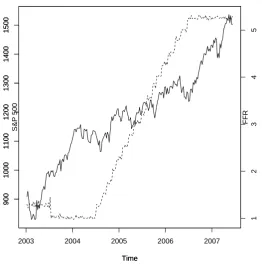
We illustrate our multivariate bubble models with an application to a data set consisting of the S& P 500 and the Federal Funds Rate (FFR). The joint behaviour of US interest rates is much studied [22]-[24] and is also of wider interest amid concern that loose US monetary policy has inflated a succession of recent bubbles [24].
The FFR is the interest rate at which depositing institutions actively trade balances held at the Federal Reserve. In particular, data published as the FFR effective rate represents the weighted averaged across all such transactions. As the rate increases it becomes more expensive for financial institutions to borrow funds. One feature of interest is whether or not the FFR increases as a symptom of wider problems with credit worthiness. In a similar vein to the original model in [1] increases in the FFR may compensate lending institutions for the Credit Risk that they bear. It is well known that such structural problems and antibubbles in the underlying can lead to dramatic increases and bubbles in the associated interest rates [19] – see the Appendix for further details.
Following a similar approach in [23] we analyse weekly data from January 2003 to June 2007. A plot of the S& P 500 and the FFR is shown below in Figure 1. Both series show a rapid growth over time consistent with earlier suggestions of a bubble in both series. Results in Table 1 give conclusive evidence of a bubble in both univariate series. This is subsequently confirmed by the bivariate bubble model in Section 2.2. Further, the test for contagion in equation (35) suggests evidence for contagion running from the FFR to the S& P 500. This would appear to confirm similar findings of debt-fuelled bubbles in [24]. In the lead in to the crisis the FFR increased as a symptom of generally decreasing credit quality in the wider financial system. This then spilled over and led to an unsustainable bubble in the US stock market.
4.2 Multivariate antibubbles
We illustrate our multivariate models for antibubbles with an application to novel data on English house prices. The data consists of house prices for 10 English regions obtained from the Nationwide building society†. Nominal house prices are then re-scaled by a GDP deflator in
†
2003 2004 2005 2006 2007
900
1000
1100
1200
1300
1400
1500
Time
900
1000
1100
1200
1300
1400
1500
Time
1
2
3
4
5
FFR
[image:9.595.164.427.158.423.2]S&P 500
Figure 1: S& P 500 (solid lines) and Federal Funds Rate (FFR) (dashed lines).
order to translate nominal prices into real prices.
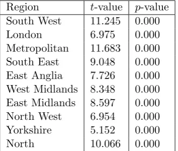
A plot of UK house prices over the period in question is shown below in Figure 2 and suggests that the antibubble that started in 2008 has been particularly severe – especially once we adjust house prices for inflation. Results shown in Table 2 below give strong statistical evidence for an antibubble in each of the ten English regions. Table 3 shows the estimated size of the antibubbles. In each region statistical evidence of an antibubble is accompanied by a significant economic effect. The impact of the antibubble splits neatly along the north-south divide – although results suggest that the East Midlands region, commonly identified as being in the South of England economically [30], should in fact be seen as part of the North of England. In the South of England house prices seem to have falled by around 1/3 in real terms. In the North of England this figure appears closer to 20%.
Univariate bubble model
t-value p-value S& P 500 162101.6 0.000 FFR 8.306 0.000
Test for contagion
[image:10.595.218.378.127.241.2]t-value p-value 22.896 0.000
Table 1: Results for the statistical tests for bubbles
2009 2010 2011 2012 2013
170000
180000
190000
200000
210000
Time
Real Pr
ice
Figure 2: English house prices 2008-2013
these cases is co-dependence rather than an asymmetric contagious effect.
5
Conclusions and further work
[image:10.595.150.433.318.578.2]Region t-value p-value South West 11.245 0.000 London 6.975 0.000 Metropolitan 11.683 0.000 South East 9.048 0.000 East Anglia 7.726 0.000 West Midlands 8.348 0.000 East Midlands 8.597 0.000 North West 6.954 0.000 Yorkshire 5.152 0.000 North 10.066 0.000
Table 2: P-values testing the null hypotheses of no anti-bubble 2008-13
Region Estimated anti-bubble component South West -0.334
[image:11.595.170.431.349.502.2]London -0.322 Metropolitan -0.370 South East -0.334 East Anglia -0.336 West Midlands -0.232 East Midlands -0.262 North West -0.208 Yorkshire -0.214 North -0.238
Table 3: Estimated size of antibubbles by English region 2008-2013
SW L M SE EA WM EM NW Y N
SW · 0.404 0.513 0.543 0.433 0.058 0.193 0.168 0.536 0.055 L 0.404 · 0.422 0.394 0.853 0.020∗ 0.046∗ 0.037∗ 0.076 0.048∗
M 0.513 0.422 · 0.891 0.564 0.019∗ 0.046∗ 0.091 0.265 0.078 SE 0.543 0.394 0.891 · 0.581 0.025∗ 0.035∗ 0.078 0.209 0.045∗
EA 0.433 0.853 0.564 0.581 · 0.028∗ 0.032∗ 0.080 0.195 0.048∗
WM 0.058 0.020∗ 0.019∗ 0.025∗ 0.028∗ · 0.899 0.781 0.227 0.825 EM 0.193 0.046∗ 0.046∗ 0.035∗ 0.032∗ 0.899 · 0.870 0.427 0.630 NW 0.168 0.037∗ 0.091 0.078 0.080 0.781 0.870 · 0.359 0.633 Y 0.536 0.076 0.265 0.209 0.195 0.227 0.427 0.359 · 0.285 N 0.055 0.048∗ 0.078 0.045∗ 0.048∗ 0.825 0.630 0.633 0.285 ·
[image:11.595.72.524.561.719.2]akin to phase-transition behaviour in statistical physics [40]. Our model highlights a possible issue with historical estimation bias. Relying on historical prices only may over-estimate gains (losses) during a bubble (antibubble), may under-estimate the true level of long-term risk and may also under-estimate long-term correlation levels potentially leading to under-diversified portfolios.
Our multivaraite models allow for a more systematic approach in empirical applications such as comparing multiple markets and evaluating contagion. Here, we can show that this leads to empirical applications that are interesting and important in their own right. The interplay between stock markets and the Federal Funds Rate (FFR) is interesting and important [22]-[24]. Firstly, we are able to show that a bubble in the FFR spills over and infects the US stock market prior to the crash of 2008. This appears to tie in closely with recent suggestions that Federal Reserve policy was directly responsible as a bubble inflated against the backdrop of decreasing lending quality [24]. Secondly, we look at the English housing antibubble that occurred from 2008-13. Evidence is found that price falls in the South Eastern part of the country “infect” the North. The often talked about North-South divide is clearly evident in English house prices. Further, results suggest that the scale of the division has been under-stated by some conventional economic approaches [30]. Allied to the above there appears to be relatively little evidence of contagion across neighbouring regions.
The bubble and antibubble models discussed in this paper are potentially very rich. Addi-tional applications include financial aspects of societal resilience [41], economic policy [42] and market psychology and trading [43]. Future work will also explore additional links with the model in [31].
Appendix: Antibubble-generated bubbles in bond yields
It is easy to show that an antibubble in the price of the underlying asset leads to a bubble in the corresponding Bond yields [19]. Following the standard approach [44] write
P(t) =M e−y(t)T, (36)
wherey(t) is the yield,T is the maturity date,M is the constant value of the bond at maturity and P(t) is the price of the underlying asset. It follows thatX(t) = lnP(t) satisfies
X(t) = lnM−y(t)T. (37)
Under the equation for an antibubble we have that
dXt=µ(t)dt+σ(t)dWt+vdj(t), (38)
where
µ(t) = µ−vh(t),
σ2(t) = σ2−v2h(t). (39)
Combining equations (37-39) it follows that the bond yields y(t) satisfy
dy(t) =−µ(t)
T dt+ σ(t)
T dW
′
t−
v
Tdj(t), (40)
where W′
t = −Wt. Thus it follows that (40) gives the formula for a speculative bubble since
W′
t d
References
[1] A. Johansen, O. Ledoit, and D. Sornette, I. J. Theor. and Appl. Financ., 3, 219 (2000)
[2] D. Sornette.Why stock markets crash: critical events in complex financial systems. (Prince-ton University Press, Prince(Prince-ton, 2003)
[3] W-X. Zhou and D. Sornette, Phys. A. 387, 243 (2008).
[4] W-X. Zhou and D. Sornette, Phys. A. 388, 869 (2009).
[5] P., Sieczka, D., Sornette, and J. A. Holyst, Eur. Phys. J. B82, 257 (2011)
[6] J. A. Feigenbaum, Quant. Financ.1, 346 (2001)
[7] J. Feigenbaum, Quant. Financ. 1, 527 (2001)
[8] G. Chang and J. Feigenbaum, Quant. Financ. 6, 15 (2006)
[9] G. Chang and J. Feigenbaum, Quant. Financ. 8, 723 (2008)
[10] D. Bree, D. Challet, D. and P.P. Perrano, Quant. Financ. 13, 275 (2013)
[11] D. Sornette, R. Woodard, W. Yan and W-X. Zhou, Physica A 392, 4417 (2013)
[12] P. Geraskin and D. Fantazzini, Eur. J. of Financ. 19, 366 (2013)
[13] L. Lin and D. Sornette, Eur. J. of Financ.19, 344 (2013)
[14] J. R. Kurz-Kim, Applied Econ. Lett.19, 1465 (2012)
[15] Z-Q. Jiang, W-X. Zhou, D. Sornette, R. Woodard, K. Bastiaensen and P. Cauwels, J. of Econ. Behav. and Organ.74, 149 (2010)
[16] D. Bree and N. Joseph, Int. Rev. of Financ. Anal.30, 287 (2013)
[17] H.M. Markowitz, Portfolio Selection: Efficient Diversification of Investments, 2nd edn. (Blackwell, Malden, Massachussets, 1971).
[18] J. Fry, Eur. Phys. J. B85, 405 (2012).
[19] J. Fry, Eur. Phys. J. B87, 1 (2014).
[20] R. Peston and L. Knight,How do we fix this mess? The economic price of having it all and the route to lasting prosperity,(Hodder and Stoughton, London, 2012)
[21] W-X. Zhou and D. Sornette, Phys. A 348, 428 (2005)
[22] W-X. Zhou and D. Sornette, Phys. A 337, 586 (2004)
[23] K. Guo, W-X. Zhou, S-W. Cheng, and D. Sornette, PLoS One 6, e22794 (2011)
[24] D. Sornette and P. Cauwels, Risks 2, 103 (2014).
[26] D. Sornette and Y. Malevergne,Extreme financial risks: From dependence to risk manage-ment. (Springer, Berlin Heidelberg New York, 2006).
[27] A. McNeil, R. Frey and P. Embrechts,Quantitative risk management. (Princeton University Press, Princeton, 2005).
[28] C. Hott and P. Monnin, J. of Real Estate and Financ. Econ. 36, 427 (2008)
[29] A. Black, P. Fraser and M. Hoesli, J. of Bus. Financ. and Account.33, 1535 (2006)
[30] R. Rowthorn, Spat. Econ. Anal.,5, 363 (2010)
[31] J. Zeira, J. of Monet. Econ.43, 237 (1999)
[32] J-P. Bouchaud, and M. Potters, Theory of financial risk and derivative pricing. From sta-tistical physics to risk management, 2nd edn. (Cambridge University Press, Cambridge, 2003).
[33] W. Yan, R. Woodard and D. Sornette, Phys. A 391, 1361 (2012).
[34] D. Sornette and A. Helmstetter, Phys. A,318, 577-591 (2003)
[35] G. Pryce and K. Gibb, Real Estate Econ.34, 377 (2006)
[36] D. R. Cox and D. Oakes,Analysis of survival data. (Chapman and Hall/CRC, Boca Raton London New York Washington D. C., 1984)
[37] J. Y. Campbell, A. Lo and J. A. C. MacKinlay,The econometrics of financial time series.. (Princeton University Press, Princeton, 1997).
[38] J. Fry, J. of Applied Res. in Financ.2, 131 (2010).
[39] D. MacKenzie and T. Spears,‘The formula that killed Wall Street?’ The Gaussian Copula and the material cultures of modelling. (Working Paper, The University of Edinburgh, 2012).
[40] L. Borland, Quant. Financ. 12, 1367 (2012).
[41] J. Coaffee,Terrorism, risk and the city. (Ashgate, Aldershot, 2003).
[42] N. Carnot, V. Koen, and B. Tissot, Economic forecasting and policy, 2nd edn. (Palgrave Macmillan, Basingstoke New York, 2011).
[43] T. Plummer,Forecasting financial markets. The psychology of successful investing. (Kogan Page, London, 2006).