Munich Personal RePEc Archive
The Diffusion of Development: Along
Genetic or Geographic Lines?
Campbell, Douglas L. and Pyun, Ju Hyun
August 2014
Online at
https://mpra.ub.uni-muenchen.de/57933/
1
The Diffusion of Development: Along Genetic or Geographic Lines?
Douglas L. Campbell¶ Ju Hyun Pyun§
New Economic School (NES) Korea University Business School
August 2014
Abstract
Why are some peoples still poor? Recent research suggests that a society’s “genetic distance”—a measure of the time elapsed since two populations had common ancestry—to the United States is a significant predictor of development even after controlling for an ostensibly exhaustive list of geographic, historical, religious and linguistic variables. We find, by contrast, that the correlation of genetic distance from the US and GDP per capita disappears with the addition of controls for geography including distance from the equator and a dummy for sub-Saharan Africa.
Keywords: Genetic Distance, Economic Development, Geography, Climatic Similarity
JEL Classification: O10, O33, O40
¶
New Economic School, and the HSE-NES International Laboratory of Russian Economic History, 47 Nakhimovsky pr., Moscow 117418, Russia, E-mail: [email protected].
§ Korea University Business School, 145 Anam-Ro, Seongbuk-Gu, Seoul 136-701, Korea, E-mail:
2
1. Introduction
Why are some peoples still poor? Economists have begun to investigate the role of
genetics in the wealth of nations. One prominent example is Spolaore and Wacziarg (2009)
henceforth SW which argues that the revolution in technological innovation which began in
Lancashire cotton textiles circa 1760 spiraled outwards first to immediate locales, then to the
whole of Britain, soon to the entire English-speaking world, and finally to other culturally and
genetically similar peoples of the world.1 Today, with the United States at the forefront of the
world technological hierarchy, SW find that distance to the United States, measured
geographically, culturally, and genetically, is a determinant of a society's level of technology and
development.
The authors argue that the significance of their genetic distance variable, a measure based
on the time elapsed since two societies existed as a single panmictic population developed by
Cavalli-Sforza et al. (1994), does not imply any direct influence of specific genes on income.
Instead they argue that genetic distance proxies a divergence in traits “biologically and/or
culturally” which provide barriers to the diffusion of technology. SW report that genetic distance
“has a statistically and economically significant effect on income differences across countries,
even controlling for measures of geographical distance, climatic differences, transportation costs,
and measures of historical, religious, and linguistic distance.”2 Were the impact of genetic
distance on development robust to an exhaustive array of geographic and other barriers, it could
be construed as evidence in favor of a direct impact of genetic distance from the US on income.
This provocative result would be interesting and important, but it would also be surprising given
that genetic distance to the US appears to be strongly correlated with geographic factors (see the
world map in Fig. 1 and Table 1). Continent dummies alone can explain nearly 70% of the
variation in genetic distance (versus a still considerable 56% of the variation in income), and a
fuller set of geographic variables explain 86% of the variation in genetic distance (vs. 72% of
income)3.
[Insert Fig. 1]
1 Three other examples are Spolaore and Wacziarg (2013 and 2014), who use the same genetic data and make a
similar argument with technology adoption, and Ashraf and Galor (2011), who look at ethnic diversity.
2
Spolaore and Wacziarg (2009), p. 469.
3 These variations come from additional regressions of genetic distance on geographic variables. The results are
3
[Insert Table 1]
We find that the evidence offered in support of the theory that genetic distance predicts
GDP per capita is sensitive to geographic controls, including latitude and a dummy variable for
sub-Saharan Africa. Our findings are consistent with the theory that the technologies developed
during the Industrial Revolution diffused first to other temperate regions of the world, where
European agricultural technology could be deployed and where the disease environment was
most favorable to European people and their institutions, technology, seeds, animals and even
germs. This is the theory developed by a long line of scholars, including Crosby (1972),
Kamarck (1976), Diamond (1992), Sachs (2001), and Gallup, Mellinger, and Sachs (1999), who
all stress the importance of climatic similarity for the diffusion of various technologies.4 In a
world with trade costs, where the stability of GDP per capita rankings across decades implies
that history matters, and where Malthusian forces have certainly been a strong historically and
are debatably still at play in some developing countries (see Clark, 2008), the nature of
agricultural technology diffusion and the historical disease environment will necessarily carry
outsized importance for development. And regardless of the mechanism, it has long been known
that countries near the equator tend to be less developed. SW themselves argue for the inclusion
of latitude as a control and express legitimate concern that sub-Saharan Africa may be driving
their results, yet they do not control for either in their regressions.5
In related research, Giuliano, Spilimbergo, and Tonon (2006, 2013) find that genetic
distance does not explain trade flows within Europe after controlling for various geographic
measures. Angeles (2012) shows that SW's genetic distance proxy is sensitive to the inclusion of
12 additional linguistic, religious, colonial, geographic and another genetic control (percentage
of population with European ancestry, not counting mestizos). While these papers also argue
against a role of genetics in economic development, the former only considers trade flows and is
4 For example, Crosby (1972) notes that European people, plants, animals, and germs all colonized areas of the
world with climates most similar to Europe (which he terms “Neo-Europes”), while Diamond (1992) argues that both diseases and agricultural technology spreads more easily east-to-west, helping to give the natives of the relatively large Eurasian landmass an advantage over more isolated areas (Africa or Australasia) and over those living in continents with a north-to-south axis such as the Americas. Kamarck (1976) discusses the extreme difficulty of transplanting agricultural technologies from temperate regions to the tropics.
4
only applied to the relatively homogenous gene pool of Europe while the latter replaces one
genetic variable with another. 6
2. Empirics
We have reproduced the baseline result from SW's Table 1, which estimates the
following equation:
, ,( )
logyi =α+β⋅geni US+Xi US ⋅ +γ GEOi⋅δ ε+ i, (1)
where logyiis the log of country i’s GDP per capita in 1995, geni US, is the genetic distance to the
US from country i, and Xi US,( ) are vectors of geographic controls from SW. Xi US,( ) includes
absolute longitudinal and latitudinal difference from the US, distance from the US, contiguity
with the US and a dummy for sharing an ocean with the US, and being an island or landlocked.
i
GEO are important climatic and geographic difference controls omitted in SW, including
distance from the equator and a dummy for sub-Saharan Africa.
In column (1) of Table 2, we find that “genetic distance to the US,” measured as the
amount of time elapsed since the populations in these countries separated, is a significant
predictor of income per capita even after controlling for various measures of physical distance.7 Yet, column (1) does not contain any variables which denote differences in climatic
endowments. “Absolute difference in latitude” from the US is included, but “absolute difference
in absolute latitude” distance from the equator8 is not. The reason why the latter is the appropriate control should be clear: although the Southern Cone countries, South Africa, and
Australasia all have very large absolute differences in latitudes with the US, they have similar
climates owing to their similar absolute latitudes with Europe and the United States.
6 The 2006 version of Giuliano et al. considers incomes, the 2013 version does not. Riahi (2013) argues that
historical settler mortality explains both genetic distance and incomes.
7
Our sample size is slightly larger than SW’s as their original sample is not publicly available and could not be acquired, and there is one variable, freight rate to the northeastern US, which we could not get as the original website listed as the source in SW appears to be no longer operable. This variable was not significant in SW, and eliminating all of SW’s other controls do not change our results (Table 1, Column 4). Our replicated coefficient is slightly larger than that in SW -- -13.5 vs. -12.5.
8
5
[Insert Table 2]
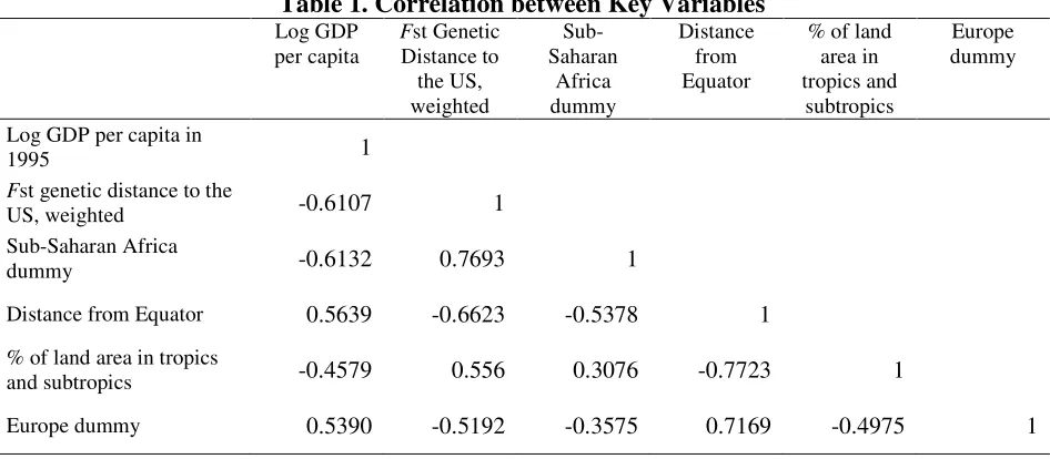
Fig. 2.A displays the nonlinear relationship between income and absolute difference in
latitude with the US that SW considers as their one of main geographic controls, while the strong
relationship between income and distance from the equator is readily apparent in Fig. 2.B. SW
themselves write that latitude could affect income directly, or via technology diffusion, and so is
a relevant control, yet they do not include distance from the equator as a control in their primary
results in SW’s Table 1 (p.488). By including distance from equator in column (2), the marginal
effect of genetic distance on income difference decreases by 33% although the genetic distance
coefficient is still significant.
[Insert Fig. 2]
In addition, Fig. 2.B captures heterogeneity of the geographic region of sub-Saharan
Africa. In Fig. 2.B, the fact that most of sub-Saharan Africa is very poor and located very close
to the equator is also apparent. It might be that "genetic distance" explains why it is that
sub-Saharan Africa is poor or why latitude is so highly correlated with development that Europeans
settled in areas with climates similar to Europe, and these places are now developed owing,
according to SW, either to the ease with which European technologies were able to diffuse to
populations with similar genetic endowments, or to the special characteristics of those
endowments.9 In column (3) of Table 2, however, when we include a dummy for the 41 sub-Saharan African nations in our sample the very first specification we tried the coefficient on
genetic distance falls substantially, rendering the results insignificant. Thus genetic distance to
the US does not seem to help explain poverty in Africa or in the tropics.10
SW presciently express concern that sub-Saharan Africa may be driving their results, but
instead of including it as a control, as is standard in the cross-country growth literature, including
Barro (1991), Fisher (1991), Sala-i-Martin (1997) and Lorentzen, McMillan, and Wacziarg
9 Bloom and Sachs (1998) emphasize the geographic and climatic characteristics of sub-Saharan Africa in
determining poor economic performance in the region, arguing that “Sub-Saharan Africa is the far most tropical in
the simple sense of the highest proportions of land and population in the tropics of the world’s major regions.” The recent works also consider various causes of poor economic performance of sub-Saharan Africa such as legacy of colonial rules and slave trading, heavy dependence on a small number of primary exports, internal politics and corruption, demographic changes, etc.
10 One may argue whether or not sub-Saharan Africa dummy represents only geographic factors of the region
6
(2008)11, SW report that their results are robust to excluding sub-Saharan Africa countries in their regressions.12 Yet, while sub-Saharan Africa is very poor and distant genetically from the US, within Africa, the richer countries tend to be genetically remote (see Fig. 3). This pattern
also holds for other regions such as Asia. In fact, several rich East-Asian nations, such as Japan,
Hong Kong, and Singapore, are actually more distant from the US genetically than many very
poor sub-Saharan Africa countries, such as Somalia, Ethiopia, and Madagascar (see Fig. 3).
Given that evidence within sub-Saharan Africa itself constitutes a clear counterexample, it is
legitimate to ask why excluding a group of counterexamples is preferable to including a control
for sub-Saharan Africa, as is the standard in the cross-country income regression literature. In
addition, SW themselves argue that the impact of genetic distance on income is robust to the
inclusion of controls for large geographic regions.
[Insert Fig. 3]
As distance from the equator is an imperfect proxy for climate, when we include a more
precise climatic variable, the percentage of each country's land area in the tropics or sub-tropics
in column (4), the point estimate falls even further. In column (5), we show that that controlling
for the tropics and sub-Saharan Africa alone eliminates the result.
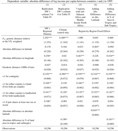
To show robustness, we also try controlling for just two continental dummies – Europe
and sub-Saharan Africa. The aforementioned cross-country growth studies conventionally
include continent dummies to show the validity of their results. Europe is rich and genetically
close to the US, and sub-Saharan Africa is poor and genetically distant from the US. The
regression results in column (6) demonstrate that, aside from this observation, the variable
genetic distance has no predictive power, as the within-region evidence is not supportive. In Fig.
4, it can be seen that there is no statistically significant correlation between GDP per capita and
genetic distance to the US outside of sub-Saharan Africa and Europe.13 Finally, in column (7),
when we expand the sample to include 20 additional countries14 for which we do not have
11 The important point is that the Sahara desert constitutes a barrier, and so is a very relevant control. As the famous
sign in Zagora, Morocco says, it takes 52 days to get to Timbuktu by camel (Encyclopedia Brittanica).
12
Spolaore and Wacziarg (2009), p. 501.
13 In Figure 4, we get a coefficient of -5.3, but with a standard error of 3.3.
7
complete data, and just include controls for Europe, sub-Saharan Africa, Asia and contiguity
(effectively a North America dummy), we again find no statistically significant relationship.15
[Insert Fig. 4]
SW also argue that if genetic distance to the US predicts income levels, then the income
differential between any two countries should be a function of their relative genetic distance to
the US. Thus, SW spend most of their paper presenting pairwise differenced regressions
(baseline controls in SW’s Table IV) showing that relative genetic distance to the US is
correlated with income differences generally. The authors difference GDP per capita at the
dyadic pair level for each combination of 137 (145 in our sample) countries, manufacturing
9,316 highly dependent data points (10,296 in our slightly larger sample), and use this as the
dependent variable with the regressor of interest now being relative genetic distance to the US.
The other regressors are differences in geographic variables for each bilateral observation. It
should be noted that if there is no cross-country relationship between genetic distance to the US
and income, then it is unlikely that relative genetic distance to the US could predict income
differentials. 16 We include our Table 3 in the interest of being thorough. The following specification is built on SW’s pairwise differenced regressions:
| log log | R X
i j ij ij ij ij
y − y =α+β⋅gen + γ +ρ +ε , (2)
where | logyi−logyj|is the absolute difference of log income per capita between countries i and
j in 1995, and the relative genetic difference variable is defined as R | , , |
ij i US j US
gen = gen −gen ,
where geni US, is the genetic distance to the US, and Xij is the vector of absolute difference in
other geographic variables between countries i and j. ρijare pair-wise continent (region) fixed
effects, and εijis the error term, which are clustered in two dimensions.
[Insert Table 3]
15 In the additional appendix, we show additional robustness results including those using alternative measures of
genetic distance. Notably, the inclusion of regional controls also renders the impact of genetic distance insignificant even when we exclude sub-Saharan African countries.
16
8
We reproduce columns (1) and (2) in Table 2 that benchmark SW's Table IV results.
These regressions might appear to support a role for genetic distance in development. However,
while SW correctly stress the importance of including continent dummies in their analysis, they
include only six regions (Asia, Africa, Europe, North America, Latin America, and Oceania) and
did not separate sub-Saharan Africa from Mediterranean North Africa. They included a set of six
dummies equal to one if both countries in a pair are on the same region and another set of six
dummies equal to one if one country belongs to a given region, and the other not. However,
using just 12 dummies for six regional pairings with 21 combinations could be problematic. For
example, the average absolute income difference between North America and Europe is much
smaller than the sum of the average absolute income difference between North America and all
other countries plus the average absolute income difference between Europe and all other
countries. SW’s method of continental dummies predicts a large income difference between
North America and Europe, which causes an upward bias on the coefficient genetic distance to
the US.
If instead we separate sub-Saharan Africa from the Mediterranean North African
countries, and include a separate dummy for each regional pairing i.e., a dummy for North
America paired with South America, and a separate dummy for South America paired with
sub-Saharan Africa for 28 fixed effects total then the impact of relative genetic distance shrinks and
loses significance. However, including these dummies does not render the “Absolute difference
in absolute latitude” or the “Absolute difference in % of land area in the tropics” variables
insignificant in columns (4) and (5), while several of the other geographic controls actually
increase in significance.
3. Conclusion
The results presented above show that genetic distance loses the ability to explain income
after the inclusion of geographic controls, including distance from the equator and a sub-Saharan
Africa dummy. Our findings provide additional evidence for the importance of climatic
endowment and regional dummy variables, if not the exact mechanism by which these variables
impact development. Future research should continue to introduce creative variables with the
9
has been such a strong force historically but there is scant evidence that the answer to this
mystery lies in our genetic differences.
References
Angeles, Luis. (2012). ‘Is there a Role for Genetics in Economic Development?’Working Papers
2012_02, Business School - Economics, University of Glasgow.
Ashraf, Quamrul and Oded Galor. (2011). ‘The ‘Out of Africa’ Hypothesis, Human Genetic
Diversity, and Comparative Economic Development’ NBER Working Paper 17216.
Barro, Robert J. (1991). ‘Economic Growth in a Cross Section of Countries’, Quarterly Journal
of Economics, 106, pp. 407-443.
Bloom, David and Jeffrey D. Sachs (1998). ‘Geography, Demography, and Economic Growth in
Africa,’ Brookings Papers on Economic Activity, 2.
Cameron, A. Colin, J. Gelbach and D. Miller. (2011). ‘Robust Inference with Multi-way
Clustering’, Journal of Business and Economic Statistics, 29, pp. 238-249.
Cavalli-Sforza, Luigi L., Paolo Menozzi, and Alberto Piazza. (1994). The History and
Geography of Human Genes. Princeton, NJ: Princeton University Press.
Clark, Gregory. (2008). A Farewell to Alms. A Brief Economic History of the World. Princeton,
NJ: Princeton University Press.
Crosby, Alfred. (1972). The Columbian Exchange: Biological and Cultural Consequences of
1492. Westport, CT: Greenwood Publishing Company.
Diamond, Jared. (1992). The Third Chimpanzee: The Evolution and Future of the Human Animal.
New York, NY: Harper Collins.
Fischer, S. (1991). Growth, Macroeconomics, and Development. In NBER Macroeconomics
Annual 1991, Volume 6 pp. 329-379.
Gallup, John L., Andrew D. Mellinger, and Jeffrey D. Sachs. (1999). ‘Geography and Economic
Development’, International Regional Science Review, 22, pp. 179-222.
Giuliano, Paola, Antonio Spilimbergo, and Giovanni Tonon. (2006). ‘Genetic, Cultural and
10
Giuliano, Paola, Antonio Spilimbergo, and Giovanni Tonon. (2013). ‘Genetic Distance,
Transportation Costs and Trade’, Journal of Economic Geography, Forthcoming.
Hall, Robert E. and Jones, Charles I. (1999) ‘Why Do Some Countries Produce So Much More
Out-put Per Worker Than Others?’ Quarterly Journal of Economics, 114(1), pp. 83-116.
Kamarck, Andrew. (1976). The Tropics and Economic Development: A Provocative Inquiry in
the Poverty of Nations. Baltimore, MD: The Johns Hopkins Press.
Lorentzen, Peter, John McMillan, and Romain Wacziarg. (2008). ‘Death and Development’,
Journal of Economic Growth, 13, pp. 81-124.
Riahi, Ideen. (2013). ‘Colonization and Genetics of Comparative Development’. Discussion
Papers dp13-11, Department of Economics, Simon Fraser University.
Sachs, Jeffrey D. (2001). ‘Tropical Underdevelopment’, NBER working paper, No. 8119.
Sala-i-Martin, Xavier X. (1997). ‘I Just Ran Two Million Regressions’, American Economic
Review, 87, pp. 178-183.
Spolaore, Enrico and Romain Wacziarg. (2009). ‘The Diffusion of Development’, Quarterly
Journal of Economics, 124, pp. 469-529.
Spolaore, Enrico & Romain Wacziarg. (2013). ‘How Deep Are the Roots of Economic
Development?,’ Journal of Economic Literature, 51(2), pp. 325-69.
Spolaore, Enrico and Romain Wacziarg. (2014). ‘Long Term Barriers to the International
Diffusion of Innovations’, in: Handbook of Economic Growth, edition 1, volume 2,
chapter 3, pp. 121-176.
11
Table 1. Correlation between Key Variables
Log GDP per capita
Fst Genetic Distance to the US, weighted
Sub-Saharan
Africa dummy
Distance from Equator
% of land area in tropics and
subtropics
Europe dummy
Log GDP per capita in
1995 1
Fst genetic distance to the
US, weighted -0.6107 1
Sub-Saharan Africa
dummy -0.6132 0.7693 1
Distance from Equator 0.5639 -0.6623 -0.5378 1
% of land area in tropics
and subtropics -0.4579 0.556 0.3076 -0.7723 1
12
Table 2. Income Level Regressed on Various Geographic Measures, 1995
Dependent variable: log income per capita, 1995
(1) SW's Baseline Controls (2) Add Distance from equator (3) Add Distance from equator & sub-Saharan Africa (SSA) dummy (4)
Add (%) of Land Area in Tropics and Sub-Tropics (5) Sparse Controls (SSA dummy & Climatic Control) (6) Two Continent Controls only (7) Enlarged Sample, with Continent Controls
FST genetic distance to
the US, weighted
-13.28*** -8.924*** -3.301 -1.261 -3.176 -3.12 -2.778
[2.061] [2.276] [2.729] [2.876] [2.724] [2.521] [2.207]
Absolute difference in latitude from US
1.811** 1.085* 1.308** 1.643***
[0.709] [0.605] [0.564] [0.619]
Absolute difference in longitude from US
1.130** 0.013 0.051 0.473
[0.490] [0.507] [0.462] [0.431]
Geodesic distance from the US (1000s of km)
-0.234** -0.029 -0.047 -0.143
[0.100] [0.103] [0.095] [0.088]
=1 for contiguity with the US
1.200*** 0.521* 0.451* 0.487* 0.948***
[0.212] [0.312] [0.246] [0.272] [0.341]
=1 if share a common sea or ocean
-0.407* 0.024 -0.102 -0.135
[0.240] [0.253] [0.251] [0.252]
=1 if the country is an island
0.656** 0.660** 0.473 0.528**
[0.315] [0.317] [0.294] [0.258]
=1 if the country is landlocked
-0.392 -0.469** -0.527** -0.517**
[0.245] [0.225] [0.226] [0.235]
Distance from the Equator
0.031*** 0.029***
[0.007] [0.007]
% of land area in tropics and sub-tropics
-1.109*** -0.740***
[0.248] [0.230]
Sub-Saharan Africa dummy
-0.940*** -1.293*** -1.277*** -1.168*** -1.362***
[0.228] [0.245] [0.270] [0.248] [0.225]
Europe dummy 0.985*** 0.736***
[0.199] [0.192]
Asia dummy -0.593**
[0.251]
Constant 9.774*** 8.294*** 8.193*** 9.480*** 9.271*** 8.713*** 8.951***
[0.267] [0.444] [0.436] [0.287] [0.190] [0.243] [0.232]
Observations 145 145 145 145 145 145 165
R2 0.447 0.503 0.541 0.552 0.46 0.496 0.489
Notes: 1. Robust Standard errors in parentheses; *significant at 10%; **significant at 5%; ***significant at 1%.
2. Genetic distance data from Cavalli-Sforza et al. (1994) via SW (2009). Geographic data is from the Centre d’Etudes Prospectives et d’Informations Internationales (CEPII), Tropics variable from Gallup, Mellinger, and Sachs available at http://www.ciesin.columbia.edu/eidata/, and GDP data is from the World Bank's WDI.
3. The genetic variable (Weighted Fst distance) is the time elapsed between two populations on average.
13
Table 3. Paired World Income Difference Regression (Two-way Clustering)
Dependent variable: absolute difference of log income per capita between countries i and j in 1995
(1) (2) (3) (4) (5)
[image:14.595.58.533.126.653.2]Replication SW’s column 5 in
Table IV
Replication SW’s column 6 in Table IV
7 regions with
sub-Saharan Africa and
Middle East& North
Africa
Adding Abs. Difference
in Abs. Latitude
Adding Abs. Difference
in % of Area in Tropics and Sub-Tropics
SW’s Regional
Dummy
Climate
control only Region-by-Region Fixed Effects
FST genetic distance relative
to the US, weighted
3.292*** 6.489*** 1.000 0.645 0.660
(1.252) [1.165] (1.141) (1.135) (1.130)
Absolute difference in latitude
-0.170 0.104 -0.031 -0.465* -0.094
(0.226) [0.264] (0.258) (0.279) (0.262)
Absolute difference in longitude 0.258* -0.02 0.467** 0.228 0.410**
(0.146) [0.182] (0.203) (0.188) (0.193)
Geodesic distance (1000s of km)
-0.027 -0.014 -0.041 -0.008 -0.036
(0.020) [0.024] (0.027) (0.025) (0.026)
=1 for contiguity
-0.339*** -0.580*** -0.359*** -0.318*** -0.339***
(0.068) [0.072] (0.070) (0.067) (0.068)
=1 for either country is island (0 for both are islands)
0.168** 0.149 0.166** 0.159* 0.156*
(0.083) [0.095] (0.082) (0.082) (0.084)
=1 for either country is landlocked (0 for both landlocked)
0.161** 0.128* 0.135** 0.153** 0.142**
(0.073) [0.075] (0.067) (0.065) (0.066)
=1 if pair shares at least one sea or ocean
0.106* -0.001 0.051 0.070 0.054
(0.054) [0.057] (0.056) (0.057) (0.055)
Absolute difference in absolute latitude
0.010***
(0.004)
Absolute difference in % of land area in tropics and subtropics
0.190* 0.183**
[0.109] (0.089)
Observations 10,296 10,296 10,296 10,296 10,296
Notes: 1. Two-way clustered standard errors in parentheses (Cameron et al. 2011). *significant at 10%; ** significant at 5%; *** significant at 1%.
2. All data are from the same sources as in Table 2.
14
Fig. 1. Chloropleth Map: Weighted Genetic Fst Distance from the US
(Darker countries are genetically relatively more distant from the US.)
Fig. 2. Latitudinal Distance from the US vs. Distance from the Equator
DZA ARG ARM AUS AUT AZE BGD BLR BEL BLZ BEN BTN BOL BWA BRA BRN BGR BFA BDI KHM CMR CAN CAF TCD CHL CHN COL COG CRI CIV CYP DNK DOM ECU EGY SLV GNQ ETH FIN FRA GAB GMB GEO GHA GRC GTM GIN GNB GUY HTI HND HUN ISL IND IDN IRN IRL ISR ITA JAM JPN JOR KAZ KEN KOR KWT KGZ LVALBN LSO LBR LTU LUX MDG MWI MYS MLI MRT MEX MDA MNG MAR MOZ NAM NPL NLD NZL NIC NER NGA NOR OMN PAK PAN PNG PRY PER PHL POL PRT ROM RUS RWA SAU SEN SLE ZAF ESP LKA SDN SUR SWZ SWE CHE SYR TJK TZA THA TGO TTO TUN TUR TKM UGA UKR ARE GBR URY UZB VEN VNM ZAR ZMB AGO ALB DJI TWN LAO SVN SVK HRV CZE ERI DEU MKD 4 6 8 1 0 1 2 L o g G D P p e r c a p it a i n 1 9 9 5
0 .2 .4 .6 .8
Absolute difference in latitude from the US
A. GDPPC vs. Difference in latitude from the US
DZA ARG ARM AUS AUT AZE BGD BLR BEL BLZ BTN BOL BRA BRN BGR KHM CAN CHL CHN COL CRI CYP DNK DOM ECU EGY SLV FIN FRA GEO GRC GTM GUY HTI HND HUN ISL IND IDN IRN IRL ISR ITA JAM JPN JOR KAZ KOR KWT KGZ LVA LBN LTU LUX MYS MEX MDA MNG MAR NPL NLD NZL NIC NOR OMN PAK PAN PNG PRY PER PHL POL PRT ROM RUS SAU ESP LKA SUR SWE CHE SYR TJK THA TTO TUN TUR TKM UKR ARE GBR URY UZB VEN VNM ALB TWN LAO SVN SVK HRV CZE DEU MKD BEN BWA BFA BDI CMR CAF TCD COG CIV GNQ ETH GAB GMB GHAGIN GNB KEN LSO LBR MDG MWIMLI MRT MOZ NAM NER NGA RWA SEN SLE ZAF SDN SWZ TZATGO UGA ZAR ZMB AGO DJI ERI 4 6 8 1 0 1 2 L o g G D P p e r c a p it a i n 1 9 9 5
0 20 40 60 80
Absolute latitude
Rest of World Sub-Saharan Africa
Fitted values
[image:15.595.73.515.440.595.2]15
Fig. 3. Income per capita vs. Genetic Distance to the US: Asia and sub-Saharan Africa
BEN BWA BFA BDI CMR CPV CAF TCD COM COG CIV GNQ ETH GAB GMB GHA GIN GNB KEN LSO LBR MDG MWI MLI MRT MUS MOZ NAM NER NGA RWA SEN SYC SLE ZAF SDN SWZ TZA TGO UGA ZAR ZMB AGO DJI ERI ARM AZE BGD BTN BRN KHM CHN GEO HKG IND IDN JPN KAZ KOR KGZ MYS MNG NPL PAK PHL RUS SGP LKA TJK THA TKM UZB VNM TWN LAO 4 6 8 1 0 1 2 L o g G D P p e r c a p it a , 1 9 9 5
.05 .1 .15 .2
Weighted Fst Genetic Distance to the US
Fitted Values, SSA Sub-Saharan Africa Fitted Values, Asia Asia
Fig. 4. . Income per capita vs. Genetic Distance to the US: World ex sub-Saharan Africa and Europe DZA ATG ARG ARM AUS AZE BHR BGD BLZ BTN BOL BRA BRN KHM CAN CHL CHN COL CRI DMA DOM ECU EGY SLV FJI GEO GRD GTM GUY HTI HND HKG IND IDN IRN ISR JAM JPN JOR KAZ KIR KOR KWT KGZ LBN MYS MEX MNG MAR NPL NZL NIC OMN PAK PAN PNG PRY PER PHL RUS KNA LCA VCT SAU SGP SLB LKA SUR SYR TJK THA TON TTO TUN TKM ARE URY UZB VUT VEN VNM WSM TWN LAO 7 8 9 1 0 1 1 L o g G D P p e r c a p it a i n 1 9 9 5
0 .05 .1 .15 .2
Weighted Fst Genetic Distance to the US
Actual Values Fitted Values (Slope Not Statistically Signficant)
[image:16.595.117.486.472.713.2]