Addressing Class Imbalance for Improved Recognition of Implicit
Discourse Relations
Junyi Jessy Li University of Pennsylvania [email protected]
Ani Nenkova University of Pennsylvania [email protected]
Abstract
In this paper we address the problem of skewed class distribution in implicit dis-course relation recognition. We examine the performance of classifiers for both bi-nary classification predicting if a particu-lar relation holds or not and for multi-class prediction. We review prior work to point out that the problem has been addressed differently for the binary and multi-class problems. We demonstrate that adopting a unified approach can significantly im-prove the performance of multi-class pre-diction. We also propose an approach that makes better use of the full annotations in the training set when downsampling is used. We report significant absolute im-provements in performance in multi-class prediction, as well as significant improve-ment of binary classifiers for detecting the presence of implicit Temporal, Compari-son and Contingency relations.
1 Introduction
Discourse relations holding between adjacent sen-tences in text play an essential role in establishing local coherence and contribute to the semantic in-terpretation of the text. For example, the causal re-lationship is helpful for textual entailment or ques-tion answering while restatement and exemplifica-tion are important for automatic summarizaexemplifica-tion.
Predicting the type of implicit relations, which are not signaled by any of the common explicit discourse connectives such as because, however, has proven to be a most challenging task in dis-course analysis. The Penn Disdis-course Treebank (PDTB) (Prasad et al., 2008) provided valuable annotations of implicit relations. Most research to date has focused on developing and refining lex-ical and linguistlex-ically rich features for the task
(Pitler et al., 2009; Lin et al., 2009; Park and Cardie, 2012). Mostly ignored remains the prob-lem of addressing the highly skewed distribution of implicit discourse relations. Only about 35% of pairs of adjacent sentences in the PDTB are con-nected by three of the four top level discourse re-lation: 5% participate in Temporalrelation, 10% inComparison(contrast) and 20% inContingency
(causal) relations. The remaining pairs are con-nected by the catch-all Expansionrelation (40%) or by some other linguistic devices (24%). Finer grained relations of interest to particular applica-tions account for increasingly smaller percentage of the PDTB data.
Class imbalance is particularly problematic for training a binary classifier to distinguish one rela-tion from the rest. As we will show later, it also impacts the performance of multi-class prediction in which each pair of sentences is labeled with one of the five possible relations.
All prior work has resorted to downsampling the training data for binary classifiers to distin-guish a particular relation and use the full train-ing set for multi-class prediction. In this pa-per we compare several methods for address-ing the skewed class distribution duraddress-ing trainaddress-ing: downsampling, upsampling and computing fea-ture weights and performing feafea-ture selection on the unaltered full training data. A major motiva-tion for our work is to establish if any of the alter-natives to downsampling would prove beneficial, because in downsampling most of the expensively annotated data is not used in the model. In addi-tion, we seek to align the treatment of data imbal-ance for the binary and multi-class tasks. We show that downsampling in general leads to the best pre-diction accuracy but that the alternative models provide complementary information and signifi-cant improvement can be obtained by combining both types of models. We also report significant improvement of multi-class prediction accuracy,
achieved by using the alternative binary classifiers to perform the task.
2 The Penn Discourse Treebank
In the PDTB, discourse relations are viewed as a predicate with two arguments. The predicate is the relation, the arguments correspond to the min-imum spans of text whose interpretations are the abstract objects between which the relation holds. Consider the following example of a contrast rela-tion. The italic and bold fonts mark the arguments of the relation.
Commonwealth Edison saidthe ruling could force it to slash its 1989 earnings by$1.55 a share. [Implicit = BY COM-PARISON] For 1988, Commonwealth Edison reported earnings of $737.5 million, or $3.01 a share.
For explicit relations, the predicate is marked by a discourse connective that occurs in the text, i.e.
because,however,for example.
Implicit relations are marked between adjacent sentences in the same paragraph. They are inferred by the reader but are not lexically marked. Alter-native lexicalizations (AltLex) are the ones where there is a phrase in the sentence implying the rela-tion but the phrase itself was not one of the explicit discourse connectives. There are 16,224 and 624 examples of implicit andAltLexrelations, respec-tively, in the PDTB.
The sense of discourse relations in the PDTB is organized in a three-tiered hierarchy. The four top level relations are: Temporal (the two argu-ments are related temporally),Comparison (con-trast), Contingency (causal) and Expansion (one argument is the expansion of the other and contin-ues the context) (Miltsakaki et al., 2008). These are the classes we focus on in our work.
Finally, 5,210 pairs of adjacent sentences were marked as related by an entity relation (EntRel), by virtue of the repetition of the same entity or topic. EntRels were marked only if no other rela-tion could be identified and they are not considered a discourse relation, rather an alternative discourse phenomena related to entity coherence (Grosz et al., 1995). There are 254 pairs of sentences where no discourse relation was identified (NoRel).
Pitler et al. (2008) has shown that performance as high as 93% in accuracy can be easily achieved for the explicit relations, because the connective it-self is a highly informative feature. Efforts in iden-tifying the argument spans have also yielded high accuracies (Lin et al., 2014; Elwell and Baldridge, 2008; Ghosh et al., 2011).
However, in the absence of a connective, recog-nizing non-explicit relations, which includes im-plicit relations, alternative lexicalizations, entity relation and no relation present, has proven to be a real challenge. Prior work on supervised implicit discourse recognition studied a wide range of fea-tures including lexical, syntactic, verb classes, se-mantic groups via General Inquirer and polarity (Pitler et al., 2009; Lin et al., 2009). Park and Cardie (2012) studied the combination of features and achieved better performance with a different combination for each individual relation. Meth-ods for improving the sparsity of lexical represen-tations have been proposed (Hernault et al., 2010; Biran and McKeown, 2013), as well as web-driven approaches which reduce the problem to explicit relation recognition (Hong et al., 2012).
Remarkably, no prior work has discussed the highly skewed class distribution of discourse re-lation types. The tacitly adopted solution has been to downsample the negative examples for one-vs-all binary classification aimed at discovering if a particular relation holds and keeping the full train-ing set for multi-class prediction.
To highlight the problem, in Table 1 we show the distribution of implicit relation classes in the entire PDTB. In our work, we aim to develop clas-sifiers to identify the four top-level relations listed in the table1.
# of samples Percentage
Temporal 1038 4.3%
Comparison 2550 11.3%
Contingency 4532 20%
Expansion 9082 40%
Table 1: Distribution of implicit relations in the PDTB.
3 Experimental settings
In our experiments, we used all non-explicit in-stances in the PDTB sections 2-19 for training and those in sections 20-24 for testing. Like most stud-ies, we kept sections 0-1 as development set. In order to ensure we have a large enough test set to properly perform tests for statistical significance over F scores and balanced accuracies, we did not follow previous work (Lin et al., 2014; Park and Cardie, 2012) that used only section 23 or sec-tions 23-24 for testing. Also, the traditional rule of thumb is to split the available data into training
and testing sets with 80%/20% ratio. Our choice ensures that this is the case for all of the relations. The only features that we use in our experiments are production rules. We exclude features that oc-cur fewer than five times in the training set. Pro-duction rules are the state-of-the-art representation for discourse relation recognition. This represen-tation leads to only slightly lower results than a system including a much larger variety of features in the first end-to-end PDTB style discourse parser (Lin et al., 2014) .
The production rule representation is based on the constituency parse of the arguments and in-cludes both syntactic and lexical information. A production rule is the parent with an left-to-right ordered list of all of its children in the parse tree (for example, S→NP VP). All non-terminal nodes are included as a parent, from the sentence head to the part-of-speech of a terminal. Thus words that occur in each sentence augmented with their part of speech are part of the representation (for example, NN→company), along with more gen-eral structures of the sentence corresponding to production rules with only non-terminals on the right-hand side.
There are three features corresponding to a pro-duction rule, tracking if the rule occurs in the parse of first argument of the relation, in the second, or in both.
Adopting this representation allows us to fo-cus on the issue of class imbalance and how the choices of tackling this problem affect even-tual prediction performance. Our findings are representation-independent and will most likely extend to other representations.
We train and evaluate a binary classifier with linear kernel using SVMLight2 (Joachims, 1999)
for each of the four top level classes of relations:
Temporal, Comparison, Contingencyand Expan-sion. We used SVM-Multiclass3for standard
mul-tiway classification. We also develop and evaluate two approaches for multiway classification for the four classes plus the additional class of entity rela-tion and no relarela-tion.
Due to the uneven distribution of classes, we use precision, recall and f-measure to measure binary prediction performance. For multiway
classifica-2http://svmlight.joachims.org/
3http://svmlight.joachims.org/svm multiclass.html
tion, we use the balanced accuracy (BAC):
BAC = 1
k k
X
i=1
ci
ni, (1)
wherekis the number of relations to predict,ciis the number of instances of relationithat are cor-rectly predicted,niis the total number of instances of relationi.
Balanced accuracy (or averaged accuracy) has a more intuitive interpretation than F-measure. It is not dominated by the majority class as much as standard accuracy is. For example for two classes, in a dataset where one class makes up 90% of the data, predicting the majority class has accuracy of 90% but balanced accuracy of 45%.
In testing, we keep the original distribution in-tact and make predictions for all pairs of adjacent sentences in the same paragraph that do not have an explicit discourse relation 4. In order to
per-form tests for statistical significance over F scores, precision, recall and balanced accuracies, we ran-domly partitioned the testing data into 10 groups. We kept the data distribution in each group as close as possible to the overall testing set. To com-pare the performance of two different systems, a paired t-test is performed over these 10 groups. 4 Why downsampling?
Binary classification As mentioned in the
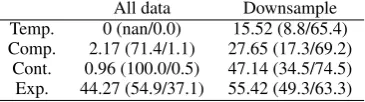
pre-vious sections, in all prior work of supervised im-plicit relation classification, the technique to cope with highly skewed distribution for binary classi-fication is to downsample the negative training in-stances so that the sizes of positive and negative classes are equal. The reason for doing so is that the classifier can achieve high accuracy just by ig-noring the small class, learning nothing and aways predicting the larger class. We illustrate this ef-fect in Table 2. Without downsampling, the only reasonable F measure is achieved for Expansion
where the smaller class accounts for 40% of the data. Note that with downsampling, the recogni-tion ofExpansionis also improved considerably.
Multiway classification In prior work multiway
All data Downsample Temp. 0 (nan/0.0) 15.52 (8.8/65.4) Comp. 2.17 (71.4/1.1) 27.65 (17.3/69.2)
[image:4.595.87.270.63.114.2]Cont. 0.96 (100.0/0.5) 47.14 (34.5/74.5) Exp. 44.27 (54.9/37.1) 55.42 (49.3/63.3)
Table 2: F measure (precision/recall) of binary classification: including all of the data vs down-sampling.
to poor results in identifying the core Temporal,
ComparisonandContingencydiscourse relations. We propose an alternative approach to multi-class prediction, based on binary one-against-all classi-fiers for each of the four discourse relations, in-cludingExpansion, trained using downsampling.
The intuition is that an instance of adjacent sen-tences Si is assigned to a discourse relation Rj if the binary classifier for Rj recognizes Si as a positive instance with confidence higher than that of the classifiers for other relations. If none of the binary classifiers recognizes the instance as a positive example, the instance is assigned to class
EntRel/NoRel. This approach modifies the way multi-class classifiers are normally constructed by including downsampling and having special treat-ment of theEntRel/NoRelclass.
Specifically, we first use the four binary classi-fiersCj for each relationjto get the confidencepj of instanceibelonging to classj. We approximate the confidence by the distance to the hyperplane separating the two classes, which SVMLight pro-vides. If at least onepjis greater than zero, assign instance i the class k where the classifier confi-dence is the highest. If none of thepj’s is greater than zero, assignito be theEntRel/NoRelclass.
We show balanced accuracies of these two mul-tiway classification methods in Table 3.
Multiway SVM One-Against-All
5-way 32.58 37.15
Table 3: Balanced accuracies for SVM-Multiclass and one-against-all 5-way classification.
The one-against-all approach leads to 5% abso-lute improvement in performance. A t-test anal-ysis confirms that the difference is significant at p < 0.05. Note that the improvement comes en-tirely from acknowledging that skewed class dis-tribution poses a problem for the task and by ad-dressing the problem in the same way for binary and multi-class prediction.
5 Using more data
Although downsampling gives much better per-formance than simply including all of the origi-nal data, it still appears to be an undesirable so-lution because in essence it throws away much of the annotated data. This means that for the small-est relations, as much as 90% of the data will not be used. Feature selection and feature val-ues are computed only based on this much smaller dataset and do not properly reflect the information about discourse relations encoded in the PDTB. In this section we first discuss some of the widely used methods for handling skewed data distribu-tion, that is, weighted cost and upsampling. First, we show that with highly skewed distributions, the two methods result in almost identical classifiers. Then we introduce a method for feature selection and shaping which computes feature weights on the full dataset and thus captures much of the in-formation lost in downsampling.
5.1 Weighted cost and upsampling
A number of methods have been developed for the skewed distribution problem (Morik et al., 1999; Veropoulos et al., 1999; Akbani et al., 2004; Batista et al., 2004; Chawla et al., 2002). Here we highlight weighted cost and random upsampling, which are known to work well and widely used.
The idea behind weighted cost (Morik et al., 1999; Veropoulos et al., 1999) is to use weights to adjust the penalties for false positives and false negatives in the objective function. As in Morik et al. (1999), we specify the cost factor to be the ratio of the size of the negative class vs. that of the positive class.
In the case of upsampling, instead of ran-domly downsampling negative instances, positive instances are randomly upsampled. In our exper-iments we randomly replicate positive instances with replacement until the numbers of positive and negative instances are equal to each other.
The binary and multiway classification results for these two methods are shown in Table 4 and Table 5. For binary classification, we can see sig-nificantly higher F score for the smallestTemporal
weighted cost, than using downsampling in one-against-all manner.
Upsample WeightCost Temp. 20.35* (16.8/25.9) 20.61* (16.9/26.3) Comp. 28.11 (20.6/44.5) 28.38 (19.9/49.6)
Cont. 46.46 (37.4/61.3) 46.36 (34.6/70.1) Exp. 54.93 (50.3/60.5) 57.43* (43.9/83.1)
Table 4: F-measure (precision/recall) of binary classification: upsampling vs. weighted cost.
For Temporal and Comparison relations listed in Table 4, we noticed an interesting similarity between the F and precision values of upsam-pling and weighted cost. To quantify this simi-larity, we calculated the Q-statistic (Kuncheva and Whitaker, 2003) between the two classifiers. The Q-statistic is a measurement of classifier agree-ment raging between -1 and 1, defined as:
Qw,u= NN11N00−N01N10
11N00+N01N10 (2)
Wherewdenotes the system using weighted cost, udenotes the upsampling system.N11means both
systems make a correct prediction, N00 means
both systems are incorrect,N10meanswis
incor-rect butu is correct, andN01 meanswis correct
butuis incorrect.
We have the following Q statistics: Tempo-ral: 0.999, Comparison: 0.9938, Contingency: 0.9746, Expansion: 0.7762. These are good in-dicators that for highly skewed relations, the two methods give classifiers that behave almost identi-cally on the test data. In the discussions that fol-low, we discuss only weighted cost to avoid redun-dancy.
5.2 Feature selection and shaping
While weighted cost or upsampling can give bet-ter performance over downsampling for some rela-tions, their disadvantages towards multi-class clas-sification and the obvious favor towards the major-ity class give rise to the following question: is it possible to inform the classifier of the information encoded in the annotation ofallof the data while still using downsampling to handle the skewed class distribution? Our proposal is feature value augmentation. Here we introduce a relational ma-trix in which we calculate augmented feature ues via feature shaping. We first compute the val-ues of features on the entire training set, then use the downsampled set for training with these val-ues. In this way we pass on to the classifiers
infor-mation about the relative importance of features gleaned from the entire training data.
5.2.1 Feature shaping
The idea of feature shaping was introduced in the context of improving the performance of linear SVMs (Forman et al., 2009). In linear SVMs the prediction is based on a linear combination of
weight×feature values. The sign ofweight indi-cates the preference for a class (positive or nega-tive), the value of the feature should correspond to how strongly it indicates that class. Thus, features that are strongly discriminative should have high values so that they can contribute more to the final class decision. Here we augment feature values for a relation according to the following criteria: 1. Features are considered “good” if they strongly indicate the presenceof the relation; 2. Features are considered “good” if they strongly indicate the
absenceof the relation; 3. features are considered “bad” if their presence give no information about
either the presence or the absenceof the relation. To capture this information, we first construct a relation matrixM with each entryMij defined as the conditional probability of relationRjgiven the feature Fi computed as the maximum likelihood estimate from the full training set:
Mij =P(Rj|Fi)
Each column of the relation matrix captures the predictive power of each feature to a certain re-lation. A feature with valueMij higher than the column mean indicates that it is predictive for the presence of relation j, while a feature with Mij lower than the mean is predictive for its absence; the strength of such indication depends on how far awayMij is from the mean: the further away it is, the more valuable this feature should be for rela-tionj. With this idea we give the following aug-mented value for each feature:
Mij0 = (
Mij, ifMij ≥µj. µj + (µj−Mij), ifMij < µj. (3)
where µj is the mean of the jth column corre-sponding to thejth relation.
feature shaping, we allow features that strongly in-dicate the absence of a class to influence the deci-sion and rely on the classifier to identify the tive association and reflect it by assigning a nega-tive weight to these features.
When constructing the relation matrix, we used the top four relation classes along with an En-tRel/NoRelclass. We computed the matrix before downsampling to preserve the natural data distri-bution and features that strongly indicate the ab-sence of a class, then downsample the negative data just like the previous downsampling setting.
5.2.2 Feature selection
The relation matrix also provides information for feature selection using a binomial test for signifi-cance,B(n, N, p), which gives the probability of observing a feature n times in N instances of a relation if the probability of any feature occurring with the relation isp. For each relation, we use the binomial test to pick the features that occur signif-icantly more or less often than expected with the relation. In the binomial test,pis set to be equal to the probability of that relation in the PDTB train-ing set. We select only the features which result in a lowp-value for the binomial test for at least some relation. We used 9-fold cross validation on the training data to pick the bestp-values for each re-lation individually; all bestp-values were between 0.1 and 0.2.
Result listing Table 5 and Table 6 show the
mul-tiway and binary classification performance using feature shaping and feature selection. We also show the precision and recall for binary classifiers.
Multiway SVM One-Against-All
AllData 32.58 NA
Downsample NA 37.15
Upsample NA 36.63
Weighted Cost NA 34.23
Selection 32.52 38.42*
Shaping NA 38.81**
Shape+Sel NA 39.13**
Table 5: Balanced accuracy for multiway SVM and one-against-all for 5-way classification. One asterisk (*) means significantly better than weighted cost and upsampling, and two means sig-nificantly better than downsampling, atp <0.05.
For multi-way classification, performing feature shaping leads to significant improvements over downsampling, upsampling and weighted cost. The binomial method for feature selection that
relies on the full training data distribution has a similar effect. Combined feature shaping and se-lection leads to 2% absolute improvement in dis-course relation recognition. For binary classifica-tion, though, the improvement is significant only forTemporal.
6 Classifier analysis and combination
6.1 Discussion of precision and recall
A careful examination of Tables 5 and 6 leads to some intriguing observations. For the most skewed relations, if we consider not only the F measure, but also the precision and recall, there is an interesting difference between the systems. While downsampling has the lowest precision, it gives the highest recall. The case for weighted cost is another story. For highly skewed relations such asTemporalandComparison, it gives the highest precision and the lowest recall; but as the data set balances out in downsampling, the classifier shifts towards high recall and low precision.
We can also rank the three feature augmentation techniques in terms of how much they reflect dis-tributional information in the training data. Fea-ture selection reflects the training data least among the three, because it uses information from all of the data to select the features, but the feature val-ues are still either 1 or 0. Feature shaping engages more data because the value of a feature encodes its relative “effectiveness” for a relation. We can see that feature selection gives slightly higher pre-cision than just downsampling; feature shaping, on the other hand, gives precision and recall val-ues between these two. This is most obvious in smaller relations, i.e.TemporalandComparison.
To see if this trend is statistically significant, we did a paired t-test over the precision and recall for each system and each relation. For theTemporal
Downsample WeightCost Selection Shaping Shape+Sel Temp. 15.52 (8.8/65.4) 20.61* (16.9/26.3) 18.47* (10.7/65.9) 20.37* (12.6/53.2) 21.30* (13.7/47.8) Comp. 27.65 (17.3/69.2) 28.38 (19.9/49.6) 26.98 (17.4/60.1) 27.79 (18.3/58.2) 26.92 (18.7/48.2)
[image:7.595.86.510.62.114.2]Cont. 47.14 (34.5/74.5) 46.36 (34.6/70.1) 47.45 (34.7/75.2) 47.62 (35.4/72.9) 46.93 (35.2/70.5) Exp. 55.42 (49.3/63.3) 57.43* (43.9/83.1) 55.52 (49.3/63.5) 55.13 (49.3/62.5) 54.90 (49.2/62.1)
Table 6: F score (precision/recall) of classifiers with feature augmentation. Asterisk(*) means F score or BAC is significantly greater than plain downsampling atp <0.05.
precision and recall with downsampling systems are not significant; yet weighted cost shifted to-wards predicting more of the positive instances, i.e., giving a significantly higher recall by trading with a significantly lower precision (p <0.05).
6.2 Discussion of classifier similarity
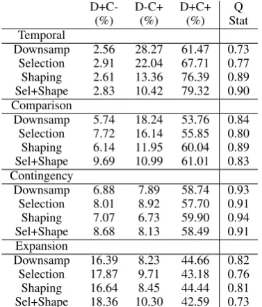
To better understand the differences of classi-fier behaviors under the weighted cost and each downsampling technique (plain downsampling, feature selection, feature shaping, feature shap-ing+selection), in Table 7 we show the percentage of test instances that the weighted cost system and each downsample system agree or do not agree. In particular, we study the following situations:
1. The downsample system predicts correctly but the weighted cost system does not (“D+C-”);
2. The weighted cost system predicts correctly but the downsample system does not (“D-C+”);
3. Both systems are correct (“D+C+”).
At a glance of the Q statistic, it seems that the systems are not behaving very differently. How-ever, as only the sum of disagreements is reflected in the Q statistic, we look more closely at where the systems do not agree in each situation. If we focus on the rarer Temporaland Comparison re-lations, first note that in the plain downsampling vs. weighted cost, the percentage of test instances in the “D+C-” column is much smaller than that in the “D-C+” column. This aligns with the above observation that plain downsampling gives much lower precision for these relations than weighted cost. Now, as more data is engaged from first using feature selection, then using feature shap-ing, then using both, the percentage of instances where both systems predict correctly increase. At the same time, there is a drop in the percentage of test instances in the “D-C+” column. This trend is also a reflection of the observation that as more data is engaged, the precision got higher as the recall drops lower. As the data gets more evenly distributed, this phenomenon fades away. The ta-ble also reveals a subtle difference between fea-ture shaping and feafea-ture selection. Compared to
D+C- D-C+ D+C+ Q
(%) (%) (%) Stat
Temporal
Downsamp 2.56 28.27 61.47 0.73 Selection 2.91 22.04 67.71 0.77 Shaping 2.61 13.36 76.39 0.89 Sel+Shape 2.83 10.42 79.32 0.90 Comparison
Downsamp 5.74 18.24 53.76 0.84 Selection 7.72 16.14 55.85 0.80 Shaping 6.14 11.95 60.04 0.89 Sel+Shape 9.69 10.99 61.01 0.83 Contingency
Downsamp 6.88 7.89 58.74 0.93 Selection 8.01 8.92 57.70 0.91 Shaping 7.07 6.73 59.90 0.94 Sel+Shape 8.68 8.13 58.49 0.91 Expansion
Downsamp 16.39 8.23 44.66 0.82 Selection 17.87 9.71 43.18 0.76 Shaping 16.64 8.45 44.44 0.81 Sel+Shape 18.36 10.30 42.59 0.73
Table 7: Q statistics and agreements (in percent-ages) of each downsampling system vs. weighted cost. “D” denotes the respective downsample sys-tem in the left most column; “C” denotes the weighted cost system. A “+” means that a system makes a correct prediction; a “-” means a system makes an incorrect prediction.
downsampling, feature selection introduces an in-crease in the column “D+C-” (i.e. the weighted cost system makes a mistake but the downsample system is correct). Feature shaping, on the other hand, do not necessarily increase this new kind of difference between classifiers.
6.3 Classifier combination
Our classifier comparisons revealed that for highly skewed distributions, there are consistent differ-ences in the performance of classifiers obtained by using the training data in different ways. It stands to reason that a combination of these classifiers with different strengths will result in an overall im-proved classifier. This idea is explored here.
[image:7.595.319.508.166.387.2]class with confidencepic. Here again we approx-imate the confidence of the class by the distance from the hyperplane dividing the two classes. We weight the two predictions and get a new predic-tion confidence by:
p0
i= αdpαid+αupic
d+αc . (4) where theαs are parameters we want to encode how much we trust each classifier. To get these values, we train the classifiers and get the accura-cies from each of them on the development set. Since we are using linear SVMs in our experi-ments, we mark the sample as positive ifpi > 0, and negative otherwise.
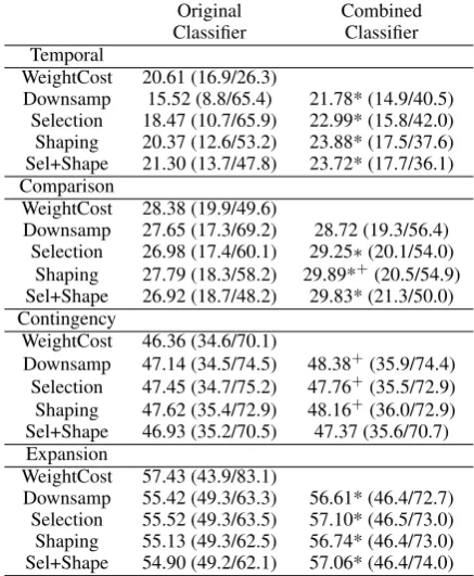
The results for the combination are shown in Ta-ble 8. We include the original performances of the classifiers by themselves for reference.
F measure ForTemporal, the combined
classi-fier performs better than the original classiclassi-fiers. We see significant (p <0.05) improvements over the corresponding downsampling system and the weighted cost system. If feature shaping is in-volved in the combination, it is also having bet-ter performance that tend toward significance (p <
0.1) over the weighted cost classifier. For Compar-ison, the benefits of a combined system is also ob-vious for feature shaping and/or selection. Feature shaping combined with weighted cost gives sig-nificantly (p < 0.05) better performance than ei-ther of them individually, and feature selection and shaping+selection combined with weighted cost is better than themselves alone. For Contingency, though weighted cost do not give better results, the improvement tends toward significance (p <0.1) when combined with plain downsampling. For Ex-pansionwhere weighted cost gives the lowest pre-cision, combination with other classifiers do not give significant improvements over F scores.
Precision and recall We can also compare the
precision and recall for each system before and af-ter combination. In all but one cases forTemporal
andComparison, we observe significantly higher precision and much lower recall after the combi-nation. The case forExpansionis just the opposite as expected.
7 Conclusion
In this paper, we studied the effect of the use of an-notated data for binary and multiway classification
Original Combined Classifier Classifier Temporal
WeightCost 20.61 (16.9/26.3)
Downsamp 15.52 (8.8/65.4) 21.78* (14.9/40.5) Selection 18.47 (10.7/65.9) 22.99* (15.8/42.0) Shaping 20.37 (12.6/53.2) 23.88* (17.5/37.6) Sel+Shape 21.30 (13.7/47.8) 23.72* (17.7/36.1) Comparison
WeightCost 28.38 (19.9/49.6)
Downsamp 27.65 (17.3/69.2) 28.72 (19.3/56.4) Selection 26.98 (17.4/60.1) 29.25∗(20.1/54.0)
Shaping 27.79 (18.3/58.2) 29.89*+(20.5/54.9)
Sel+Shape 26.92 (18.7/48.2) 29.83* (21.3/50.0) Contingency
WeightCost 46.36 (34.6/70.1)
Downsamp 47.14 (34.5/74.5) 48.38+(35.9/74.4)
Selection 47.45 (34.7/75.2) 47.76+(35.5/72.9)
Shaping 47.62 (35.4/72.9) 48.16+(36.0/72.9)
Sel+Shape 46.93 (35.2/70.5) 47.37 (35.6/70.7) Expansion
WeightCost 57.43 (43.9/83.1)
[image:8.595.306.525.62.328.2]Downsamp 55.42 (49.3/63.3) 56.61* (46.4/72.7) Selection 55.52 (49.3/63.5) 57.10* (46.5/73.0) Shaping 55.13 (49.3/62.5) 56.74* (46.4/73.0) Sel+Shape 54.90 (49.2/62.1) 57.06* (46.4/74.0)
Table 8: Classifier combination results for binary classification. An asterisk(*) means significantly better than the corresponding downsampling sys-tem at, and a plus(+) means significantly better than weighted cost, at p < 0.05. Improvements that tend toward significance (p < 0.1) are not shown here but are discussed in the text.
References
Rehan Akbani, Stephen Kwek, and Nathalie Japkow-icz. 2004. Applying support vector machines to imbalanced datasets. InMachine Learning: ECML 2004, pages 39–50.
Gustavo E. A. P. A. Batista, Ronaldo C. Prati, and Maria Carolina Monard. 2004. A study of the behavior of several methods for balancing machine learning training data. ACM SIGKDD Explorations Newsletter - Special issue on learning from imbal-anced datasets, 6(1):20–29, June.
Or Biran and Kathleen McKeown. 2013. Aggregated word pair features for implicit discourse relation dis-ambiguation. In Proceedings of the 51st Annual Meeting of the Association for Computational Lin-guistics (ACL): Short Papers, pages 69–73.
Nitesh V. Chawla, Kevin W. Bowyer, Lawrence O. Hall, and W. Philip Kegelmeyer. 2002. SMOTE: Synthetic minority over-sampling technique. Jour-nal of Artificial Intelligence Research, 16(1):321– 357, June.
R. Elwell and J. Baldridge. 2008. Discourse connec-tive argument identification with connecconnec-tive specific rankers. InIEEE International Conference on Se-mantic Computing (IEEE-ICSC), pages 198 –205. George Forman, Martin Scholz, and Shyamsundar
Ra-jaram. 2009. Feature shaping for linear SVM classi-fiers. InProceedings of the 15th ACM International Conference on Knowledge Discovery and Data Min-ing (KDD), pages 299–308.
Sucheta Ghosh, Richard Johansson, Giuseppe Ric-cardi, and Sara Tonelli. 2011. Shallow discourse parsing with conditional random fields. In Pro-ceedings of the 5th International Joint Conference on Natural Language Processing (IJCNLP), pages 1071–1079.
Barbara J. Grosz, Scott Weinstein, and Aravind K. Joshi. 1995. Centering: A framework for model-ing the local coherence of discourse. Computational Linguistics, 21:203–225.
Hugo Hernault, Danushka Bollegala, and Mitsuru Ishizuka. 2010. A semi-supervised approach to im-prove classification of infrequent discourse relations using feature vector extension. InProceedings of the 2010 Conference on Empirical Methods in Natural Language Processing (EMNLP), pages 399–409. Yu Hong, Xiaopei Zhou, Tingting Che, Jianmin Yao,
Qiaoming Zhu, and Guodong Zhou. 2012. Cross-argument inference for implicit discourse relation recognition. InProceedings of the 21st ACM Inter-national Conference on Information and Knowledge Management (CIKM), pages 295–304.
Thorsten Joachims. 1999. Making large-scale support vector machine learning practical. In Advances in kernel methods, pages 169–184.
Ludmila I. Kuncheva and Christopher J. Whitaker. 2003. Measures of diversity in classifier ensembles and their relationship with the ensemble accuracy. Machine Learning, 51(2):181–207, May.
Ziheng Lin, Min-Yen Kan, and Hwee Tou Ng. 2009. Recognizing implicit discourse relations in the Penn Discourse Treebank. In Proceedings of the 2009 Conference on Empirical Methods in Natural Lan-guage Processing (EMNLP), pages 343–351. Ziheng Lin, Hwee Tou Ng, and Min-Yen Kan. 2014. A
PDTB-styled end-to-end discourse parser. Natural Language Engineering, 20:151–184, 4.
Eleni Miltsakaki, Livio Robaldo, Alan Lee, and Ar-avind Joshi. 2008. Sense annotation in the Penn Discourse Treebank. In Proceedings of the 9th International Conference on Computational Lin-guistics and Intelligent Text Processing (CICLing), pages 275–286.
Katharina Morik, Peter Brockhausen, and Thorsten Joachims. 1999. Combining statistical learning with a knowledge-based approach - a case study in intensive care monitoring. InProceedings of the Six-teenth International Conference on Machine Learn-ing (ICML), pages 268–277.
Joonsuk Park and Claire Cardie. 2012. Improving im-plicit discourse relation recognition through feature set optimization. InProceedings of the 13th Annual Meeting of the Special Interest Group on Discourse and Dialogue (SIGDIAL), pages 108–112.
Emily Pitler, Mridhula Raghupathy, Hena Mehta, Ani Nenkova, Alan Lee, and Aravind Joshi. 2008. Eas-ily identifiable discourse relations. In Proceed-ings of the International Conference on Computa-tional Linguistics (COLING): Companion volume: Posters, pages 87–90.
Emily Pitler, Annie Louis, and Ani Nenkova. 2009. Automatic sense prediction for implicit discourse re-lations in text. InProceedings of the Joint Confer-ence of the 47th Annual Meeting of the ACL and the 4th International Joint Conference on Natural Language Processing of the AFNLP (ACL-IJCNLP), pages 683–691.
Rashmi Prasad, Nikhil Dinesh, Alan Lee, Eleni Milt-sakaki, Livio Robaldo, Aravind Joshi, and Bonnie Webber. 2008. The Penn Discourse TreeBank 2.0. InProceedings of the Sixth International Conference on Language Resources and Evaluation (LREC). Konstantinos Veropoulos, Colin Campbell, and Nello