Providing and Analyzing NLP Terms for our Community

Providing and Analyzing NLP Terms for our Community

Gil Francopoulo Tagmatica

[email protected]

Joseph Mariani LIMSI-CNRS [email protected]

Patrick Paroubek LIMSI-CNRS

[email protected]

Frédéric Vernier Paris-Sud U. - LIMSI-CNRS

[email protected].

Abstract

By its own nature, the Natural Language Processing (NLP) community is a priori the best equipped to study the evolution of its own publications, but works in this direction are rare and only recently have we seen a few attempts at charting the field. In this paper, we use the algo-rithms, resources, standards, tools and common practices of the NLP field to build a list of terms characteristic of ongoing research, by mining a large corpus of scientific publications, aiming at the largest possible exhaustivity and covering the largest possible time span. Study of the evo-lution of this term list through time reveals interesting insights on the dynamics of field and the availability of the term database and of the corpus (for a large part) make possible many further comparative studies in addition to providing a test field for a new graphic interface designed to perform visual time analytics of large sized thesauri.

1 Introduction

In the NLP community, we have tools, algorithms, resources, standards and common practices, but do we have a good knowledge of the terms that we use? The work we present here is an attempt at improving the situation. Our corpus contains articles from NLP conferences and journals about written, spoken and for a relatively small part, signed language processing, which is to our knowledge the largest ever collected in our field. It covers a time period from 1965 to 2015 and holds approximately 65,000 papers. Using OCR and PDF converters, we extracted the textual content of the documents and linked it into a database1 _{with cleaned metadata about the associated events. After an NLP analysis of the content by} means of lemmatizing, syntactic parsing, Named Entity recognition and various semantic lexical filtering with both large sized general language resources and some domain related ones, we produced a database of community specific terms which was manually checked. The result is a collection of terms annotated with various attributes like document-authors first appearance, alternative forms, occurrence statistics along different dimensions, including time, conferences etc. which is made available to the community along with the public part of the corpus for further comparative studies and enhancements. In the next two sections, we present related works and our corpus. Then we describe in detail the preprocessing applied to the corpus and the term extraction process. With the resulting term database, we present a study about “creation” (first appearance of a term in the corpus) and “impact” (relative dominance of a term in the last year of the time period covered by the corpus), introducing on this occasion a dedicated graphic interface designed for visual time analytics of large sized thesauri. Before concluding, we provide some interesting insights on the global dynamics of our field, revealed by the evolution of a few characteristic terms.

2 Situation with respect to other studies

The approach is to apply NLP tools on texts about NLP itself, taking advantage of the fact that we have a good knowledge of the domain ourselves. In the past, a similar methodology has been applied in the fields of applied linguistics (Nazar, 2011) and lexicography (deSchryver, 2012).

1_{The term database is freely available at http://www.nlp4nlp.org/resultsOfRunsGlobal/}

allinnovators.html

Our work goes after the various studies initiated in the Workshop entitled: “Rediscovering 50 Years of Discoveries in Natural Language Processing” on the occasion of ACL 50th anniversary in 2012 (Radev et al., 2013) where a group of researchers studied the content of the corpus recorded in the ACL Anthology (Bird et al., 2008). Various studies, based on the same corpus followed, for instance (Bordea et al., 2014) on trend analysis and resulted in systems such as Saffron or the Michigan University web site. Other studies were conducted specifically on the speech-related ISCA archive (Mariani et al., 2013), and on the LREC archives (Mariani et al., 2016). More focused on resource usage is the study conducted by the Linguistic Data Consortium (LDC) team whose goal was, and still is, to build a language resource (LR) database documenting the use of the LDC resources (Ahtaridis et al., 2012).

3 Corpus

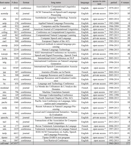
The corpus NLP4NLP2 _{is made of the largest possible selection of NLP papers from conferences and} journals, covering written, speech and for a limited part, sign language processing sub-domains; reach-ing out to a limited number of sub-corpora for which Information Retrieval and NLP activities intersect, reflecting the fact that we use NLP methods to process NLP content. It currently contains 65,003 doc-uments coming from various conferences and journals. This is a large part of the existing published articles in our field, apart from workshop proceedings and published books. Despite the fact that they often reflect innovative trends, we decided not to include workshops as they may be based on various reviewing processes and because accessing their content is often difficult. The time period spans from 1965 to 2015. Broadly speaking and aside from the small corpora intersecting neighboring domains, one third comes from the ACL Anthology3_{, one third from the ISCA Archive}4 _{and one third from IEEE}5_. The details are presented in table 1.

4 Preprocessing

Most of the papers are PDF documents and for a good part of them metadata are in various inconsistent formats. A phase of preprocessing is therefore needed to represent the various sources in a common format. We followed the organization of the ACL Anthology with distinct information groups for each document: the metadata and the content. For the former, we face four different types of sources with different format flavors and character encodings: BibTeX (e.g. ACL Anthology), custom XML (e.g. TALN), database downloads (e.g. IEEE) or HTML program of the conference (in general the program of the conference, e.g. TREC). The metadata (author names and title of each article) were normalized (java programs) into a common BibTeX format encoded in UTF8 and indexed by year and sub-corpus (conference or journal). Concerning the content, we face different possible formats, even inside the same sub-corpus as editing practices sometimes changed over time. Given that the amount of documents is huge, we cannot assign each file type individually by hand. Except for the small set of papers which where originally represented in raw text, we designed a type/subtype detection module as the first step in our normalization pipeline.

The vast majority of the documents are in PDF format of different sub-types. First, we use PDFBox6 to determine the sub-type of the PDF content: text representation or bitmap image. For the first case, we use PDFBox again to extract the text, possibly with the use of the "Legion of the Bouncy Castle"7_to extract encrypted contents. For the second case (bitmap image), we use PDFBox to extract the images and apply Tesseract OCR8 _{to transform the images into a textual content. Note that we tested some} commercial OCR but the quality improvement which was marginal did not justify its use. Then two filters are applied filter out degraded text content as sometimes the proceedings of conferences contains short abstracts of invited presentations or the OCR did not manage to extract proper content:

2_{http://www.nlp4nlp.org/} 3_{http://aclweb.org/anthology}

4_{www.isca-speech.org/iscaweb/index.php/archive/online-archive} 5_{https://www.ieee.org/index.html}

6_{https://pdfbox.apache.org/download.cgi} 7_{https://www.bouncycastle.org}

Table 1: Details of the sub-corpora. (5) In the global count of last line, for a joint conference (which is a rather infrequent situation), the papers are counted once (giving 65,003), so the sum of all cells in the table is slightly more important (yielding 67,937). Similarly, the number of venues is 558 when the joint conferences are counted once, but 577 when all venues are counted. Note that the * of the sixth column indicates inclusion in the ACL Anthology.

1. The content should be at least 900 characters.

Then we apply a set of symbolic rules to extract the abstract, body and reference sections (in XML). Using our OOV text quality indicator we were able to test alternative strategies. The first experiment was to use ParsCit9 _{(Council et al., 2008) with the original parametrization, but result were not satisfying,} especially for accented Latin strings, or Arabic and Cyrillic characters because we did not have the time to retrain the software. We also tried Grobid10_{, but we did not succeed to run it correctly with Windows} operating system. We also considered Pdfminer11_{, but it cannot deal with OCR and encrypted materials.} A semi-automatic cleaning process is applied on the metadata in order to avoid false duplicates12 concerning middle names (e.g. for a three part name like X Y Z, is Y a second given name or the first part of the family name?). To answer this kind of question we dig into the metadata when it is in a specific BibTex format, which separates the given name from the family name with a comma. Then typographic variants (e.g. "Jean-Luc" versus "Jean Luc" or "Herve" versus "Hervé") were searched and false duplicates were normalized in order to be merged, resulting in 48,894 number of different authors. Let’s add that figures are not extracted because we are unable to process and compare images. The majority (90%) of the documents comes from conferences, the rest from journals. The overall number of words is roughly 270M. Initially, the texts are in four languages: English, French, German and Russian. The number of texts in German and Russian is less than 0.5% , so they are detected automatically and discarded. The texts in French are a little bit more numerous (3%), and are kept with the same status as the English ones. This is not a problem since our pipeline is able to process both English and French.

5 Term extraction

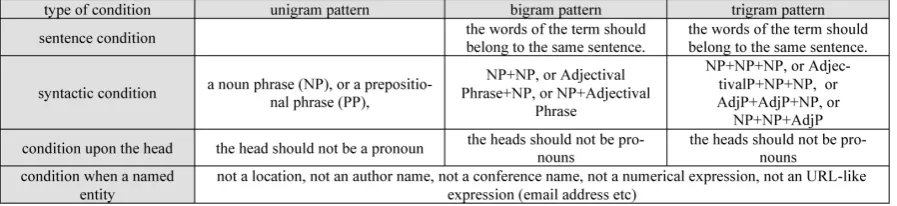
The aim is to extract the domain terms from the bodies of the texts. We used a “contrastive strategy” where we contrast a specialized corpus with a non-specialized one using salient relative term frequency deviations from their expected mean value, along the same approach as in TermoStat (Drouin, 2004). The main idea is to discard words from “ordinary” language which are not interesting for our purpose and to retain only the domain terms. Two large non-specialized, corpora, one for English, one for French are parsed with TagParser. The English corpus is made of the British National Corpus (aka BNC), the Open American National Corpus (aka OANC), the Suzanne corpus release-5 and the English EuroParl archives (years 1999 until 2009) with 200M words. The French corpus is Passage-court with 100M words13_{. These results are filtered with the syntactic patterns presented in table 2, as follows.}

Table 2:Syntactic patterns

A phase of filtering is then applied with a list of 800 unigram stop-words in order to discard various units and mathematical variables coming mainly from tables and formulas that are difficult to filter out. A small set of 30 bigram stop-words is also used to reject expressions like: “adjective adjective”. The resulting parse trees are then flattened, retaining only lemmas and excluding punctuations. Finally two statistical matrices are built, one for each language. Texts from the NLP4NLP corpus are then parsed and contrasted with this matrix according to the same syntactic patterns and conditions. Afterwards, we

9_{https://github.com/knmnyn/ParsCit} 10_{https://github.com/kermitt2/grobid} 11_{https://pypi.python.org/pypi/pdfminer}

proceed in two steps: first, we extract the terms and we analyze the 2,000 most frequent ones in order to manually merge a small amount of synonyms which are not in the parser dictionary. Then the extraction pipeline is run a second time with the finalized term list to index all their occurences.

6 Basic results

There are 3.5M of different terms totalling 24M of occurrences of these terms. For all events, the propor-tion of single words terms is always less than the one of multiword terms (70% on average), with LREC exhibiting the largest difference between the two ratios (26.6% single words versus 73.5% multiwords). In general, there are common nouns, as opposed to rare proper names like “wordnet” or “wikipedia”.

term variants of all sorts nb of occurrrences rank

NP NPs, noun phrase, noun phrases 1969140 1

HMM HMMs, Hidden Markov Model, Hidden Markov Models, Hidden Markov model, Hidden Markov models, 1950226 2 hidden Markov Model, hidden Markov Models,hidden Markov model, hidden Markov models

LM LMs, Language Model, Language Models, language model, language models 1935840 3 SR ASR, ASRs, Automatic Speech Recognition, SRs, Speech Recognition, 1928588 4

automatic speech recognition, speech recognition

POS POSs, Part Of Speech, Part of Speech, Part-Of-Speech, Part-of-Speech, Parts Of Speech, 1864532 5 Parts of Speech, Pos, part of speech, part-of-speech, parts of speech, parts-of-speech

parser parsers 1753427 6

annotation annotations 1693523 7

classifier classifiers 1642774 8

segmentation segmentations 1173835 9

dataset data-set, data-sets, datasets 1101070 10

Table 3:Basic results: the 10 most frequent terms over 1965-2015.

The 10 most frequent terms over the whole history are presented in table 3. We distinguish the classic notion of the occurrences of a term in a document from the notion of its presence, which is the number of documents holding at least one occurrence of the term. Not surprisingly, the most frequent term is “Noun Phrase“ just followed by “Hidden Markov Model”, since it is widely used by all NLP sub-communities, probably because of the linear aspect of written and spoken language.

7 Evolution over time

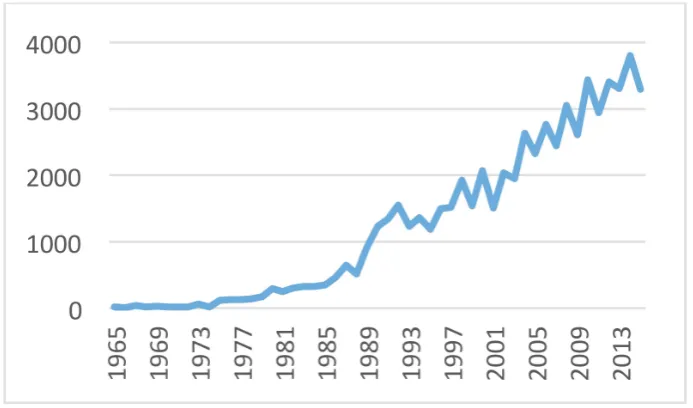
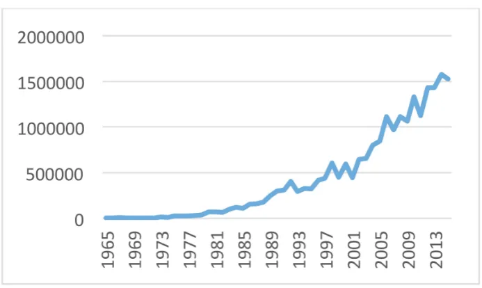
In the 60’s and the 70’s the number of documents per year was very low, but it went over 1,000 per year in the 90’s to reach 3,000 in 2015 (see figure 1). The number of term occurrences followed more or less the same shapecurve, as presented in figure 2. We can notice also the regular biennial variation in the recent years due to the fact that COLING and LREC take place every even year.

Figure 2: Occurence counts

8 Results according to creation and impact

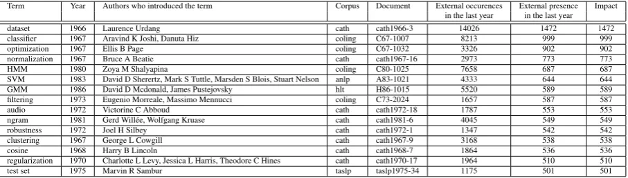
These basic figures are computed over the whole history of our domain and are of course interesting for historical purposes but they also show which terms are ruling our community today. We consider that the year, in which we observe the apparition in the corpus of the first occurrence of a term, is the “innovation year”14_{for the term. Accordingly, all the authors who use that term in their articles during} the innovation year are considered as the innovator(s) for the term. All the papers of the innovation year which hold at least one occurrence of the term are considered “innovative” papers for the term. We qualify as “external” the use of a term by authors other than the innovator(s). This distinction is important in order to exclude the overuse of particular program systems or resource names or systems specific to a particular group of people and to attribute more weight to the natural spreading of the given term rather than promote self-use by the innovator(s). The current impact of a term is defined as the number of external presences during the last year (i.e. 2015) divided by the number of innovative papers. Let’s notice that for the 15 top ranking terms in impact value, the number of innovative papers is one, so the presence in the last year is equal to the impact. The impact is therefore the measure of the relative “importance” of a term today, which is used to compute an “innovation” factor for each author (Mariani et al., 2016). The 15 “technical“ terms with top impact value are presented in table 4. Note that the present study considers for a single term all the observed form variations, but we assume that the term is used consistently throughtout the whole corpus with the same meaning, thus missing the possible cases of polysemy.

9 Visualization

Visualizing a large dataset is always a challenging task and our data raise several interesting questions. The term frequencies varies widely across time but no more than what is usually reported in other lan-guage studies. The first challenge is the aggregation of terms over different years because proceedings gather research contributions that are written many months before the official dates of the conferences, very often the year before in case of re-submissions. The second challenge is the huge numbers of spe-cialized terms used by researchers. The third challenge is presented Zipf’s law (very few terms appear frequently and most of the terms have small and comparable frequencies). However even low frequency terms remain of interest at every year because of the possible future evolution of their frequency.

Term Year Authors who introduced the term Corpus Document External occurences External presence Impact in the last year in the last year

dataset 1966 Laurence Urdang cath cath1966-3 14026 1472 1472

classifier 1967 Aravind K Joshi, Danuta Hiz coling C67-1007 8213 999 999

optimization 1967 Ellis B Page coling C67-1032 3326 902 902

normalization 1967 Bruce A Beatie cath cath1967-16 2973 773 773

HMM 1980 Zoya M Shalyapina coling C80-1025 7658 687 687

SVM 1983 David D Sherertz, Mark S Tuttle, Marsden S Blois, Stuart Nelson anlp A83-1021 4333 644 644 GMM 1986 David D Mcdonald, James Pustejovsky hlt H86-1015 5520 589 589 filtering 1973 Eugenio Morreale, Massimo Mennucci coling C73-2024 1657 587 587

audio 1972 Victorine C Abboud cath cath1972-18 1787 553 553

ngram 1981 Gerd Willée, Wolfgang Kruase cath cath1981-6 4045 549 549

robustness 1972 Joel H Silbey cath cath1972-1 1347 542 542

clustering 1967 George L Cowgill cath cath1967-9 3168 538 538

cosine 1968 Harry B Lincoln cath cath1968-7 1864 536 536

regularization 1970 Charlotte L Levy, Jessica L Harris, Theodore C Hines cath cath1970-17 1964 510 510

test set 1975 Marvin R Sambur taslp taslp1975-34 1175 501 501

Table 4:Terms with highest impacts.

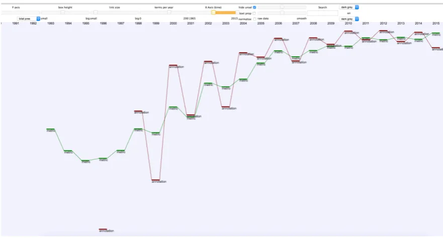
To tackle those three challenges we designed an interactive visualization called GapChart15 _where every term frequency is mapped in a graph where the x-axis represents time. GapChart uses the y-axis in a less traditional way. It mixes term frequency value (higher values displayed on top) and term ranking among other terms (lower rank displayed on top). The goal of the mix is to untangle terms with very similar frequencies on a particular year. Contribution of rank to the y-axis is computed in order to exactly spread the boxes of two consecutives terms and avoid overlapping. Gapchart provides a much cleaner view of dense/similar time series, the individual count and frequency values are not explicitly displayed but can be read by hovering the mouse pointer over a particular box. However the vertical gaps between boxes represent term frequency differences, consequently it is easy to identify visually which terms have a frequency higher than average. We added a set of interactive tools (sliders) to let the end-user zoom and move along the time axis and to control the box size, the links and the number of terms displayed. Terms can be selected by mouse click or search box and are then highlighted for analysis using a set of different colors. Also, we have added a checkbox to decide whether frequencies are normalized every year (between top and bottom of the view) or if they are normalized over the whole dataset. GapChart provides inherently cleaner display than line graphs, nevertheless the resulting visualization remained sometimes difficult to read since a small change of frequency between years can dramatically modify the ranking of a term. To solve this problem, we propose a last but not least feature: data smoothing. We first implemented a standard Gaussian blur processing where every value is replaced by a weighted average of the value and its neighbors. The system offers the possibility to manipulates the radius of the Gaussian kernel to let the user decide of the amount of smoothing applied. Pre-tests revealed that this feature is very powerful and efficient to unclutter the resulting view, but it may also hide many important features of the graph like peaks or yearly recurrent patterns. We thus found an interesting solution with a bilateral filtering, which is an improved Gaussian blur processing, also taking into account the difference of values using the same exponential formula. The second radius of this bell shaped kernel is also left adjustable to the end-user decision by means of a 5th slider.

10 Global analysis of the data

We analyzed the evolution of the terms over the period covered using the computation of the occurrences and presences and the GapChart visualization means. We first selected the terms we wanted to study, searched for their existence in the 50x200-boxes graph at some time over the 50-year timescale and allocated a different color for each of them. We then hid all other terms and reduced the time scope on the x-axis to the years when the terms occur and the ranking scope on the y-axis to the ranks of the terms according to their evolution. We then adjusted occurrence versus presence, ranking versus frequency or relative presence16_{, and experimented data smoothing with standard or bilateral filtering} Gaussian blur. Figure 3 gives an example for the set of terms “HMM” (Hidden Markov Models), “GMM” (Gaussian Mixture Models), “Neural Networks”, “DNN” (Deep Neural Networks), “RNN” (Recurrent

15_{GapChart is available athttp://newcol.free.fr/rankvis/}

Neural Networks) and “dataset”17_{, based on smoothed frequency with Gaussian blur.}

Figure 3: Evolution over time of the ranking of the terms HMM (red), GMM (blue), Neural Networks (dark green), DNN (light green), RNN (olive green) and dataset (purple) based on smoothed frequency with Gaussian blur.

Figure 4: Evolution over time of the ranking of the terms “annotation” (red) and “metrics” (green) based on smoothed frequency with bilateral filtering Gaussian blur.

We see that the first apparitions of the term “HMM” among the 200 most frequent terms occurs in the mid 80’. The term became rapidly very popular and stayed as such until the early 2010’. It was rejoined by “GMM” at the turn of the century. Neural Networks came by the end of the 80’ and became also

popular but stayed below HMMs and then GMMs. Recently progress of computation and storage al-lowed for the development of Deep Neural Networks (DNN) which appeared abruptly and rapidly joined the highest rankings. Recurrent Neural Networks (RNN) are now following and the use of “datasets” accompanies those approaches. Interestingly, we found that the term “dataset” which has the highest impact was introduced in the NLP community in the “Computer & the Humanities” journal as early as 1966 by (Urdang, 1966), who mentions“The definitions were then divided into 158 subject fields, like physics, chemistry, fine arts, and so forth. Each unit of information—regardless of length–was called a dataset, a name which we coined at the time. (For various reasons, this word does not happen to be an entry in The Random House Dictionary of the English Language, our new book, which I shall refer to as the RHD.)”.Another phenomenon may be analyzed on the terms “annotation” and “metrics” (figure 4). Here we ended using smoothed relative presence with bilateral filtering Gaussian blur.

We were surprised to see “annotation” fluctuating over the years, starting with a big increase in 1998 and reaching the highest rankings in agreement with the success of the data driven approaches and the necessity of disposing of annotated language resources. The highest rankings on those fluctuations ap-pear on even years. A possible explanation is that it is due to the impact of the LREC conferences, which are devoted to Language Resources and Evaluation and happen on even years since 1998. Similarly the term “metrics”, strongly attached to the evaluation of language technologies follows a similar evolution until it becomes a general term strongly attached to the research advances in the field and not only to the specific sub-field covered by LREC. Interestingly, the prediction of terms for future years predicts the continuation of the success of “Deep Neural Networks” and of the even years fluctuations of “annotation” (Francopoulo et al., 2016).

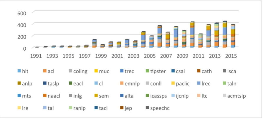
Instead of considering a set of names and all sub-corpora of NLP4NLP, another way to proceed is to select a term, starting from its first mention and to present its evolution, year after year, within the various corpora. Let’s consider “WordNet”, starting in 1991 in figure 5, which uses a classical visualization tool.

Figure 5:Evolution of "WordNet" presence in all corpora over time.

11 Conclusion

In this paper, we presented an experiment of terminology mining, by applying algorithms, resources, standards18_{, tools and common practices of the NLP field to a large sized representative sample of the} scientific literature of the NLP field itself. We have shown that NLP analysis of the text content of the scientific articles, extracted from the published electronic media, and associated with validated metadata can produce a term database with time information that provides useful insights about the dynamics of

the ongoing research in the community. In addition to showing the usefulness of lemmatizing, syntactic parsing, Named Entity recognition and various semantic lexical filtering with general and dedicated language resources for synthesizing information and saving manual cross-reference and normalization work, we have developped a specific graphic interface GapChart, especially designed for visual time analytics of large sized thesauri and delivered the terms of the domain of NLP covering both written and speech sub-domains and extended to a limited number of corpora, for which Information Retrieval and NLP activities intersect. We hope that the term database we have produced will be useful to our community for the point of view it offers upon our field and for providing the incentive to do further research on the terminology and language in NLP scientific publications.

References

Eleftheria Ahtaridis, Christopher Cieri and Denise DiPersio. 2012. LDC Language Resource Database: Building a Bibliographic Database. Proceedings of Eighth LREC, Istanbul, Turkey, ACL Anthology: L12-1549. Steven Bird, Robert Dale, Bonnie J Dorr, Bryan Gibson, Mark T Joseph, Min-Yen Kan, Dongwon Lee, Brett

Powley, Dragomir R Radev and Yee Fan Tan. 2008. The ACL Anthology Reference Corpus. A Reference Dataset for Bibliographic Research in Computational Linguistics. Proceedings of the Sixth LREC, Marrakech, Morocco, ACL Anthology: L08-1005.

Georgeta Bordea, Paul Buitelaar and Barry Coughlan. 2014. Hot Topics and schisms in NLP: Community and Trend Analysis with Saffron on ACL and LREC Proceedings. Proceedings of the Ninth LREC, Reykjavik, Iceland, ACL Anthology: L14-1697.

Issac G Councill, Giles C Lee and Min-Yen Kan. 2008. ParsCit: An open-source CRF reference string parsing package.Proceedings of the Sixth LREC, Marrakech, Morocco, ACL Anthology: L08-1291.

Patrick Drouin. 2004. Detection of Domain Specific Terminology Using Corpora Comparison. Proceedings of the Fourth LREC, Lisbon, Portugal, ACL Anthology: L04-1041.

Gil Francopoulo. 2008. TagParser: well on the way to ISO-TC37 conformance. Proceedings of the First Interna-tional Conference on Global Interoperability for Language Resources, Hong Kong, PRC, pp 82-88.

Gil Francopoulo, Frédéric Marcoul, David Causse and Grégory Piparo. 2013. Global Atlas: Proper Nouns, from Wikipedia to LMF, in LMF Lexical Markup Framework Editor G. Francopoulo, ISTE Wiley.

Gil Francopoulo, Joseph Mariani and Patrick Paroubek 2016. Predictive Modeling: Guessing the NLP Terms of Tomorrow Proceedings of LREC 2016, 23-28 May 2016, Portorož, Slovenia.

Joseph Mariani, Patrick Paroubek, Gil Francopoulo and Marine Delaborde. 2013. Rediscovering 25 Years of Dis-coveries in Spoken Language Processing: a Preliminary ISCA Archive Analysis.Proceedings of the Fourteenth Annual Conference of the International Speech Communication Association (Interspeech), Lyon, France. Joseph Mariani, Patrick Paroubek, Gil Francopoulo and Olivier Hamon. 2016. Rediscovering 15+2 Years of

Discoveries in Language Resources and Evaluation. Language Resources and Evaluation 50:165-220.

Rogelio Nazar 2011. Estudio diacrónico de la terminología especializada utilizando métodos cuantita-tivos: ejemplo de aplicación a un corpus de lingüística aplicada Revista Signos, vol.44 no.75 Valparaíso, Chile. http://www.scielo.cl/scielo.php?script=sci_pdf&pid=S0718-09342011000100005& lng=es&nrm=iso&tlng=es

Dragomir R Radev, Pradeep Muthukrishnan, Vahed Qazvinian, Amjad Abu-Jbara. 2013. The ACL Anthology Network Corpus. Language Resources & Evaluation, 47:919–944.

Gilles-Maurice de Schryver 2012. Lexicography in the Crystal Ball: Facts, Trends and Outlook R.V. Fjeld & J.M. Tor-jusen (eds.), Proc. of the 15th EURALEX International Congress, 7-11 August, 2012, Oslo: 93–163. Oslo: Department of Linguistics and Scandinavian Studies, University of Oslo. http://www.euralex.org/elx_proceedings/ Euralex2012/pp93-163%20de%20Schryver.pdf