ASH CC Algo : Coin Change Algorithm Optimization

ASH CC Algo.: Coin Change Algorithm Optimization

Ashar Mehmood

School of Electrical Engineering and Computer Science (SEECS) National University of Science and Technology (NUST)

Islamabad, 44000, Pakistan

ABSTRACT

The Coin Change problem is to represent a given amount V with fewest number of coins m. As a variation of knapsack problem, it is known to be NP-hard problem. Most of the time, Greedy alogrithm (time complexity O(m), space complexity O(1)), irrespective of real money system, doesn’t give optimal solution. Dynamic algorithm (time complexity O(mV), space complexity O(V)) gives optimal solution but is still expensive as amount V can be very large. In this paper, we have presented a suboptimal solution for the coin change problem which is much better than the greedy algorithm and has accuracy comparable to dynamic solution. Moreover, comparison of different algorithms has been stated in this paper. Proposed algorithm has a time complexity of O(m2f) and space complexity of O(1), where f is the maximum number of times a coin can be used to make amount V. It is, most of the time, more efficient as compared to dynamic algorithm and uses no memoization, this is a significant advantage over dynamic approach.

General Terms

Theory of computation, Design and analysis of algorithms, Algorithm design techniques, Dynamic programming

Keywords

Dynamic programming, Coin change problem, optimization methods, Algorithm design and analysis.

1.

INTRODUCTION

Dynamic programming (DP) [1, 2] is one of the several methods for solving different problems in computer science (and operation research). One of the distinguishing features of dynamic programming algorithm is the way it decomposes a problem into subproblems. A problem of size N decomposes to several subproblems; each of the subproblems has size N-1. Then each of which decomposes to several subproblems of size N-2, etc. Once it reaches at the lowest stage where problem is divided into many simplest subproblems, then it solves each of those subproblems just once. To avoid recomputation of same subproblems, a DP algorithm just makes records of the solution to all subproblems it encounters. In this way, at the expense of extra memory, a DP algorithm reduces the time required to solve a problem.

A dynamic programming algorithm is most appropriately applied to those problems for which table, containing the computed solutions of encountered subproblems; helps eliminate a great number of redundant computations. DP is primarily applicable to those problems that can be expressed as a sequence of decisions to be made at each of several stages. There are many dynamic programming algorithms [3] used to solve real life problems such as knapsack algorithm (for different knapsack problem [4]), Needleman–Wunsch algorithm [5], Bellman–Ford algorithm [6] etc.

Most of the usage of dynamic programming is in the field of optimization. A dynamic programming algorithm checks all the previously computed subproblems and combines their solution to give the best one. In comparison, a greedy algorithm examines the solution as some sequence of steps and chooses the solution which seems best at that instance (locally). Using a greedy algorithm one could not guarantee the globally optimal solution. Because choosing locally optimal solution may result in bad global solution.

Dynamic programming ensures the optimal solution of the given problem. Dynamic programming originated with the work of Bellman and has been applied to problems in operation research, economics, control theory, computer science and several other areas. Not surprisingly, the literature on the dynamic programming is enormous.

The proposed algorithm in this paper is of change making problem. The change making problem is an NP-hard problem [7] specifies the question of finding minimum number of coins that add up to given amount of money. It is a knapsack type problem. It has applications wider than just currency. Coin change algorithm is one of the well-known algorithms of dynamic programming. It is widely used in distributing change problem in vending machines and shipping systems etc. The algorithm proposed in this paper is an improvement over existing coin change algorithms. Unlike existing dynamic programming’s solution to coin change problem [8], the proposed algorithm does not keep any record of solution to sub problems. It updates the optimal solution at real time. Thus, in this way no extra memory is required (to keep record of solutions to all sub problems). Unlike Greedy algorithm [9], most of the time it gives the optimal solution as dynamic and the accuracy of suboptimal solutions are comparable to dynamic solution. It takes more or less same iterations and execution time to dynamic approach.

2.

DESCRIPTION

The coin change problem arises from the situation: in a shop, the cashier needs change for several transactions of money based on some coins C={cm,…,c3,c2,c1} such that

cm>…>c3>c2>c1 (in descending order) where ci denotes the ith

type of coin in C.

Formally, the Coin-Change problem solves the following integer programming problem with respect to given amount of V.

Min

s.t =V, ci>=0

Generally, representation of V under C is called the feasible solution (n1, n2, n3, . . . , nm) of the above integer programming

problem. If this representation satisfies

<ci for 2≤i≤m,

then, it is the greedy representation of V, denoted by GRDC(V), and |GRDC(V)|= is its size. Similarly, the

optimal solution (x1, x2, x3, . . . , xm) is called the optimal

representation of V, denoted by OPTC(V), and |OPTC(V)|= is its size, all mentioned in [10]. Following the aforementioned approach, the presented algorithm’s solution (a1, a2, a3, . . . ,am) is called the

suboptimal representation of V, denoted by ASHC(V), and |ASHC (V)|= is its size, where ai is the frequency (the

maximum number of times a coin ci is used to make amount V) of coin at ith denomination.

Using the presented approach, we will be able to achieve the result |ASHC(V)|, which will be equal to |OPTC(V)| in most of the time and have accuracy comparable to |OPTC(V)| in rest of the cases. But the positive point is that we use minimum space using this approach. Using minimum space we are achieving optimal result in most of the time.

We are dividing the algorithm into three parts:

 Check all the coins.

 Check maximum frequency (the maximum number of times a coin ci is used to make amount V) of each coin in making amount V and use only few of them which is enough to reach the optimal result.

 On the basis of minimum to maximum frequency (that has been used) of a specific coin, check all the other coins’ frequency in making amount V. All the aforementioned steps are done in nested form.

 for each Ci in C s.t 1≤i≤m, where m=total number of

coins in C.

 for each Ci in C  evaluate fmax.

 fmin to fminx of Ci  evaluate fCj s.t 1≤j≤m and j≠i,

where fminx≤fmax: frequencies of coin which

participate in finding optimal result.

All the aforementioned steps cover most of the cases to find optimal solution. For each frequency of each coin, the result will be updated. At the end, we will have optimal solution (|ASHC(V)|= |OPTC(V)|) or suboptimal solution having accuracy comparable to |OPTC(V)|.

3.

EXISTING TECHNIQUES

We ask that authors follow some simple guidelines. In essence, we ask you to make your paper look exactly like this document. The easiest way to do this is simply to download the template, and replace the content with your own material. Recursion [11][12] is used in the majority of programming problems as it is believed to be an efficient approach. Generally, recursion should only be used when the number of recursive calls is not excessive. The number of recursive calls somewhat depends on the amount of memory available. Stack

sizes can now be several megabytes of memory, which allows recursion to go fairly deep without causing a core dump. Sometimes recursion is used because it employs a simpler process as compared to the iterative version. For example, nearly all code written for tree-like structures is recursive. Many sorting algorithms are more naturally written recursively as well.

However, recursive solutions can be very inefficient, if one is not diligent. For example, the obvious recursive solution to compute the Nth Fibonacci number has exponential running time, even though the loop version runs in O(n) and same case is for coin change problem. Recursive formula for solving coin change problem is given below:

3.1

Algorithm

If V == 0, return 0; rsltINT_MAX; from coinsi to coinsm If (coinsi<=V)

sbrsltmin_Coin(coins[],m,V-coinsi); if (sbrslt!=INT_MAX and sbrslt+1 < rslt) rsltsbrslt+1;

return result;

Using recursive formula, the time complexity of coin change problem becomes exponential. If we consider the complete recursion tree given below then we can see that many sub problems are solved repeatedly and redundantly. It results in unnecessary overhead due to which the complexity of algorithm ends up in exponential value.

Fig 1: Recursive tree for understanding the working of recursion in coin change problem solution and its

redundant calculations [13]

Dynamic Programming is an algorithmic technique which is usually based on a recurrent formula and one (or multiple) initial state(s). A sub-solution of the problem is constructed from previously solved ones. Dynamic programming

solutions have a polynomial complexity which assures a much faster running time than other techniques like backtracking[3], brute-force[14,15], recursion etc. Algorithm of dynamic programming based solution is given below:

3.2

Algorithm

for i = 1 to V tableiINT_MAX

if (coink<=j)

sbrslttablei-coin[j]

if(sbrslt!=INT_MAX and sbrslt+1< tablei)

tableisbrslt+1

return tableV

Like other Dynamic Programming problems, recomputing the same sub problems can be avoided by constructing a temporary array table[][] in bottom up manner. But using this technique, we need memory to record all the sub-solutions. This means that the more the value of amount V to be made, the more memory overhead we will have, for the memoization. For example: consider a problem where 3 coins m (12,5,1) are used to make V (15), the dynamic approach can take up to 45 iterations and 15 memory locations, to keep record of sub-solution, to obtain the optimal result. Real life problems are far more complex and can have value V in millions and number of coins can be much greater as well. As time complexity of dynamic approach is O(mV), execution time will be large and large memory will be required to reach optimal solution.

Other than aforementioned solution, more work has also been done in this area e.g canonical coin system [10] for different types of coins or when will greedy and dynamic approach give the same optimal result (necessary conditions for canonical coin systems).

4.

PRESENTED APPROACH

Presented algorithm further optimizes the existing algorithms. It takes more or less same iterations as dynamic solution to reach a decision. For example, in above mentioned problem where coins were m(12,5,1) and we had to make V(15), more or less 30 iterations and no memory overhead are taken to reach the optimal or suboptimal solution which is drastic improvement in performance when compared to the available solutions.

In algorithm, abbreviations of different variables are used which includes Of : outputflag, Mc : min_no_of_coins, Tc : total_coins, IA : instant_val_of_amount, Am : amount and Nc : no_of_coins.

4.1

Algorithm

Ash_change(Nc,coins<vector>, Am) Offalse;

Mc0; Tcinfinite; IA0; from ci to cm

from cfmin to cfminx

Mcf;

IAAm-( ci * Mc );

if (IA==0) Oftrue; else from cj to cm

if(IA>=cj && j!=i)

McMc +(IA/cj);

IAIA%cj;

if(IA==0) Oftrue; break;

if(Tc>Mc && Of==true) TcMc;

Mc0; Offalse; IA0; return Tc;

4.2

Description

Presented algorithm, on the basis of each coin’s specific frequency, is calculating other coins’ frequencies in obtaining a specific amount (value V). It compares the frequency of the coin under consideration against the rest one by one to reach the optimal solution.

In presented algorithm,

Infinite : can be maximum value of range of data type being used to check whether amount is made or not with given coins. If it’s not made then just return data type range max value.

“Outputflag”: A flag variable to ensure that amount (value V) has made with given coins.

“Min_no_of_coins”: Minimum number of coins on the basis of a coin’s specific frequency (temporary minimum number of coins to make amount (value V)).

“total_coins”: Overall minimum number of coins (best option) needed to make amount (value V).

“Instant_val_of_amount”: A temporary variable used to represent instant value of amount.

“Amount”: Amount (V) to be made. “Ci”: coin selected at that instant

“Cm”: coin which has lowest denomination (assumed that

coins are placed in descending order) where m is total number of coins provided.

“Cj”: coin selected at that instant other than Ci.

“f”: frequency of selected coin used in making amount V. “Cfmin”: minimum frequency of selected coin used, in making

amount V i.e 0.

“Cfmax”: maximum frequency of selected coin used, in making

amount V.

“Cfminx”: frequencies which participate in obtaining optimal

result.

4.3

Logical point of view

optimal result, can be considered. It does not check some of the possible frequencies of selected coin because using those frequencies may result in bad solutions e.g it’s better to neglect those frequencies of selected coin.

On the basis of different frequencies of selected coin, it evaluates other coins’ frequencies using greedy approach. Whenever all the frequencies of other coins are calculated with respected to specific frequency of selected coin, our result is updated on the condition that the current result is smaller than or equal to previous one. Otherwise, result will retain its previous value. With combination of some frequencies of every coin and greedy approach, we are achieving optimal solution in most of the time and suboptimal solution of accuracy comparable to dynamic solution in rest of the cases.

4.4

Algorithmic point of view

We have three loops e.g outer loop, inner loop and most inner loop. Outer and most inner loop will run m (total no. of coins) times and on the basis of selected coin in outer loop, inner loop will run cfminx times (the number of times a coin

participates in obtaining optimal result).

In outer loop, algorithm checks each coin one by one and passes it to inner loop. Inner loop finds the cfmax and iterates

from cfmin to cfminx (check frequencies of selected coin which

is sufficient for obtaining optimal result.Criteria for sufficiency is described below in the example). At the end, most inner loop, on the basis of selected coin’s specific frequency, evaluates other coins’ frequencies using greedy approach but excluding the coin which is already selected in outer loop. At any moment, in most inner loop, when the amount V is reached, algorithm doesn’t check rest of the coins. It just breaks out of the loop, updates the total_coins and iterates for other frequencies of selected coin, if they exist.

With every inner loop’s iteration, total_coins is updated on condition that min_no_of_coins calculated is smaller than total_coins (instantaneous best result). This means that we update our result whenever we come up with better solution. For example, consider the case where there are coins in descending order of denominations 9, 6, 5 and 1 and we have to make amount V=11. The optimal result from dynamic approach gives 2 coins but it is done after memorization. Presented approach will find the same result without making use of memoization. Algorithm will find the best decision as given the manner that follows:

Criteria for sufficiency: Value obtained by multiplying frequency of selected coin and selected coin denomination should be less than the denomination of coin before it e.g ci*f<ci-1. Sufficiency principle will not be used for first coin

(no coin exists before it). Sufficiency principle will be followed for the coins which are factors of amount V but not strictly as mentioned above; it just also checks the selected coin maximum frequency along with frequencies which resulted from sufficiency principle (there are high chances that the maximum frequency of this coin is our optimal result).

total_coinsinfinity

On the basis of coin of denomination 9: CfmaxV/ci1

As there is no coin before 9 so it will be used maximum number of times (sufficiency principle will not be applicable in case of first coin). Its maximum frequency in making

amount V(which is 11) is 1, but if in some other case maximum frequency of first coin is greater than 1, then it will be used maximum frequency times rather than using sufficiency principle which results in a frequency lesser than maximum frequency.

We can use 9 only one time in making 11. So, inner loop will run 2 times in this branch (once for coins of denomination 9 with frequency 0 and once for frequency 1, same process will be used for all coins) and remaining amount will be made using rest of the coins in most inner loop.

fi0,1

V’V-(ci*fi)11,2

for each cj in C

min_no_of_coin=V’/cj s.t V’>cj and j!=i (eq. 1)

V’=V’%cj (eq. 2)

So, we will have 2 solutions in this branch i.e 1(6)+1(5)2 and 1(9)+2(1)3, where V is original amount and V’ is instantaneous amount. Thus, we will go for 2 coins..

As, min_no_of_coin<total_coins total_coins2

On the basis of coin of denomination 6: Cfmax V/ci1

We can use 6 only one time in making 11. So, inner loop will run 2 times in this branch and remaining amount will be made using rest of the coins in most inner loop.

fi0,1

V’V-(ci*fi)11,5

Same steps will be evaluated, aforementioned for coin of denomination 9, represented as eq.1 and eq.2. We will have 2 solutions in this branch e.g 1(9)+2(1)3 and 1(6)+1(5)2. As min_no_of_coin is not lesser than total_coins the result will remain the same.

total_coins2

On the basis of coin of denomination 5: Cfmax V/ci2

We can use 5 two times in making 11. So, inner loop should run 3 times in this branch to check all the cases but inner loop will run two times due to sufficiency principle because for frequency 2 of selected coin (denomination 5) value will be greater than the denomination of coin right before it (which is 6). However, its advantage is not observable in such cases where it discards just one iteration: its advantage is more evident in next branch (coin of denomination 1). Thus, after using frequency 0 and 1 of selected coin, remaining amount will be made using rest of the coins in most inner loop. fi0,1

V’V-(ci*fi)11,6

Same steps will be evaluated, aforementioned for coin of denomination 9, represented as eq.1 and eq.2. We will have two solutions in this branch e.g 1(9)+2(1)2 and 1(5)+1(6)2. However, neither of the two is less than total_coins current value which is 2. So, total_coins value will remain unchanged.

Cfmax V/ci11

We can use coin of denomination 1 eleven times in making 11. But this is also the case where sufficiency principle (lessen the iterations to reach optimal result) is used which says:

“We can achieve optimal result without checking all the possible frequencies of selected coin in making amount V. We use only those frequencies of selected coin whose multiplication with the selected coin is smaller than the denomination of coin right before it (coin which has next larger denomination). Use of values (resulting from multiplication of frequencies of selected coin with selected coin’s denomination) which are larger than the denomination of coin before the selected coin can lead to a bad result. Using 1 as the frequency of coin having larger denomination is better than using larger frequency of coin(s) of smaller densomination.”

For example, it’s better to use 1 coin of denomination 3 than 3 coins of denomination 1. So, if we have a coin of denomination 3 before 1 then we don’t have to check frequency 3 or 4 of coin of denomination 1, we will use 1 coin of 3 and a coin of 1 to make amount 4. However, it’s not a hard and fast rule. It’s an approximation which is done to lessen the iterations to reach the result. Thus, using sufficiency principle, inner loop, instead of running 12 times, will run only 6 times.

f0,1,2,3,4,11

Frequency 11 is used after applying sufficiency principle because 1 is the factor of amount V (which is 11). There is a chance that the maximum frequency of a coin, whose denomination is the factor of amount V, is our best result. For frequencies 0, 1, 3 and 4 amount will not be made because after using 9, 6 or 5, coin of denomination 1 cannot be used as it’s already selected. Thus, instantaneous amount cannot be made using coins of denomination 9, 6 and 5 (greedy approach is followed in most inner loop). Thus, solution for this branch will be based on frequencies 2 and 11.

f2,11

V’V-(ci*fi)9,0

Same steps will be evaluated, aforementioned for coin of denomination 9, represented as eq.1 and eq.2. We will have two solutions in this branch e.g 2(1)+1(9)3 and 11(1)11. However, none of these is less than current value of total_coins which is 2. Hence the value of total_coins will remain unaffected. So, we have traversed all the coins and their participated frequency and the result comprised of these frequencies. The total_coins is updated with every participated frequency of every coin. It can be noticed that we do not have to memoize the sub-solutions. At the end, we have our optimal result (|ASHC(V)| or total_coins for amount 11 which is equal to |OPTC(V)| which is also 2.

5.

COMPARISON

Using recursive formula the time complexity becomes exponential. It computes a same result again and again whenever it comes. It doesn’t do any memoization, which results in a large execution time. If we take three coins (12,5,1) and amount V=15 then it requires approximately 148 iterations. So, the execution time will be very large.

Dynamic programming based solution is far better than recursive formula because it uses memoization but it is still expensive e.g if we take above example in dynamic

programming solution then it takes almost 45 iterations. Alot of memory is required to record all the sub-solution. The larger the amount is, greater will be the the required memory for memoization. Outer loop runs V (amount to be made V=15) times and inner loop runs m (total no. of coins m=3) times. It makes a table of size amount V for the memoization.Thus, its time complexity and space complexity become O (mV) and O (V) respectively.

Presented algorithm’s complexity depends on the number of coins (m) and their frequency (f), in making amount V. It does not depend on the amount V to be made. If we take above example (coins {12, 5, 1}, V=15) in presented algorithm then it only takes more or less 30 iterations to make the amount (Value V). It does not need any memoization to reach the optimal or suboptimal result which is an explicit improvement in performance.

6.

EXPERIMENTAL ANALYSIS

To measure the efficiency of presented algorithm against different well known algorithms I have designed some tests which covers nearly all types of data. The test has been performed on author’s laptop and the specifications of laptop are given below:

Table 1. Author’s laptop specifications

Dell Inspiron 15 3542

Processor Intel Pentium 3558U

Core Dual Core Processor

1.7GHz, Core i3

Storage 1 TB, 5400 rpm

System memory 4GB DDR3-1600

Graphic card (integrated) Intel HD Graphics 4400

Abbreviations of different variables are used in the test which includes, NOS: Number of optimal Solutions, NSOS: Number of suboptimal Solutions, TC: Total coins needed, AVGVR: Average variation of suboptimal solutions with optimal solutions, TI: Total iterations, Algo: Algorithm used, Dyn : Dynamic approach, Pre : Presented approach, Gre : Greedy approach.

The specification and result of different test are as follow: If we consider the real money system by taking coins={1000,500,100,50,20,10,5,2,1} and amount range from 200000 to 210000 (10001 test cases), efficiency of different algorithms can be differentiated by the following table:

Table 2.0. Real money system

Algo. NOS NSOS TC AVG

VR TI

Dyn. 10001 0 10001 0 1.8*1010

Pre. 10001 0 10001 0 1.0*107 Gre. 10001 0 10001 0 9.0*104

division etc are considered an operation. Operational analysis of above test is given below:

Abbreviations of different variables are used in the test which includes, TO: Total number of operations used for whole testing, AVGOP: Average number of operation used in whole testing, MAXOP: Maximum number of operation used in whole testing.

Table 2.1. Real money system (Operational analysis)

Algo. TO AVGOP MAXOP

Dyn. 1.8*109 _{183790 1.4*10}7

Pre. 1.0*108 10212 1.4*104

Gre. 8.4*106 842 8.8*102

It is evident through operational analysis that Dynamic algorithm takes more operations than presented algorithm to compute optimal result. Thus, we can say that in this case presented algorithm is more efficient as compared to dynamic algorithm in terms of time complexity.

In real money system, greedy algorithm gives optimal solution with fewer number of iterations. But when we move towards non-real money systems and other cases then it gives very bad result.Following are some more different types of test cases which depicts the efficiency of presented algorithm over other algorithms.

Analysis of different algorithms with coins C={993,888,763,603,537,491,312,289,98,76,3,1}

(irrespective of real money system) and amount ranges from 200000 to 210000(10001 test cases) is given below:

Table 3.0. Coin, irrespective of real money system

Algo. NOS NSOS TC AVG

VR TI

Dyn. 10001 0 2081596 0 2.4*1010 Pre. 3984 6017 2090428 1.46 9.5*106 Gre. 541 9460 2180404 10.44 1.2*105

If we consider the above table it is obvious that when we move towards non-real money system then greedy approach fails to produce feasible result. Most of the time, it gives suboptimal result of very low accuracy as compared to optimal result. While if we consider presented algorithm, most of the time, it produces optimal result and accuracy of its suboptimal solution with optimal solution is very high e.g variation is just 1 (approx.)

We can notice visible difference in the efficiency of presented algorithm against greedy and dynamic approach in operational analysis, which is given below:

Table 3.1. Coins, irrespective of real money system (Operational analysis)

Algo. TO AVGOP MAXOP

Dyn. 1.6*109 155222 1.8*107

Pre. 1.1*108 10621 1.1*104

Gre. 8.7*106 872 9.6*102

Followings are the analysis of different algorithms with no. of coins C nearly equal to amount to be made. Amount ranges from 2000 to 2500 (501 test cases) and coins are 1 to V(amount)-1 e.g for V=10 coins are {1, 2, 3, 4, 5, 6, 7, 8, 9}.

Table 4.0. Number of coinsAmount to be made

Algo. NOS NSOS TC AVG

VR TI

Dyn. 501 0 1002 0 3.2*109

Pre. 501 0 1002 0 7.5*106

Gre. 501 0 1002 0 2.5*106

Considering above table we can say that greedy approach can also give optimal result in this case. In some tests, due to large number of coins, presented algorithm takes a bit more iterations than dynamic approach to find the optimal result, which can be neglected because it is a very rare case e.g number of coins m are very large (approaches to amount V to be made). Operational analysis of this case is given below:

Table 4.1.Number of coinsAmount to be made (Operational analysis)

Algo. TO AVGOP MAXOP

Dyn. 6.9*108 694193 3.2*107

Pre. 1.0*109 1003470 1.4*107

Gre. 8.0*103 8 8.0*100

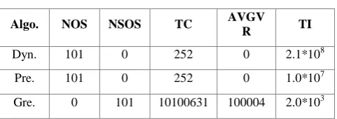
Following are the analysis of different algorithms with 20 coins and their denominations are nearly half of the amount to be made. Amount ranges from 200000 to 200100 (101 test cases) and coins are (V/2)+20 to (V/2)-18 with decrement of 2 and a coin of denomination 1 e.g for V=100, coins are {70, 68, 66, 64, . . . , 52, 50, . . , 36, 34 , 32 , 1}.

Note: Coin of denomination 1 is taken so that amount is made with any case.

Table 5.0. Coins’ denominationsV/2

Algo. NOS NSOS TC AVGV

R TI

Dyn. 101 0 252 0 2.1*108

Pre. 101 0 252 0 1.0*107

Gre. 0 101 10100631 100004 2.0*103

In above mentioned case, greedy approach totally fails to give optimal solution but if we consider presented algorithm, it gives optimal solution in all test cases with fewer number of iterations than dynamic approach. Operational analysis of this case is given below:

Table 5.1.Coins’ denominationsV/2 (Operational analysis)

Algo. TO AVGOP MAXOP

Dyn. 1.5*109 15303700 1.5*107

Pre. 3.5*108 _{3501770 3.5*10}6

Following are the analysis of different algorithms with very small no. of coins where the difference in their denominations is very large. Amount ranges from 1000 to 21000 (20001 test cases) and coins C = {449, 93, 1}.

Table 6.0. Fewer coins, larger difference

Algo. NOS NSOS TC AVGV

R TI

Dyn. 10001 0 4746584 0 6.1*109

Pre. 10001 0 4746584 0 1.0*107 Gre. 1783 8218 5026316 34.03 3.0*104

Considering above case, it is obvious that greedy approach gives infeasible result in such cases too. While, presented algorithm gives optimal solution in all test cases with fewer number of iterations than dynamic approach. Operational analysis of this case is given below:

Table 6.1.Fewer coins, larger difference (Operational analysis)

Algo. TO AVGOP MAXOP

Dyn. 1.8*109 189370 5.0*106

Pre. 1.3*108 13279 1.3*104

Gre. 2.0*107 2010 2.2*103

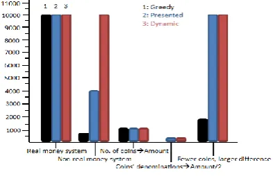
Following are the graphs of optimal solution and average number of operations in each set of test cases.

Fig 2: No. of optimal solutions in each set of test cases

Fig 3: Average no. of operations needed in each set of test cases

Thus, It can be clearly noticed after all the analysis that greedy approach works fine for the real money system but if we move towards non-real money system and other cases, it gives infeasible solutions. On the other hand, if we consider

performance of presented approach by analyzing both graphs, presented approach gives optimal solution in almost every set of test cases except non-real money system. In non-real money system, its solution varies with a small proportion to optimal solution e.g just 2, 3 coins more needed. Now, look at the average number of operations needed for each set of test cases. Iteration has not been used as criteria because of the reason that there can be many operations in an iteration of an algorithm than other algorithm’s iteration. It can be noticed that in few set of test cases, such as the set of test cases where no. of coins approaches to amount to be made, presented algorithm takes more operations than dynamic approach to find the result. But again, such cases are very rare. The main advantage of presented approach is that all the optimal and suboptimal solutions are evaluated using O(1) space. Unlike dynamic approach, no memoization has been done to find the result. Therefore, it is a big advantage to use proposed algorithm over dynamic approach.

7.

COMPLEXITY ANALYSIS AND ITS

COMPARISON

We ask that authors follow some simple guidelines. In essence, we ask you to make your paper look exactly like this document. The easiest way to do this is simply to download the template, and replace the content with your own material. This paper hasn’t presented a thorough complexity analysis of the presented approach but some cases have been discussed which clearly distinguish its uses and outline its benefits over other approaches. In worst case, algorithm checks almost every coin in most inner loop and considers most of the possible frequencies of selected coin in inner loop (discarding few frequencies). The problem will be in worst case when every coin of larger denomination is very far from its consecutive smaller coin (larger difference in their denominations). Thus, outer loop runs m (number of coins) times and for every coin in outer loop, inner loop runs nearly fmax (every possible frequency to make amount V) times. However, it does not iterate fmax number of times because of sufficiency principle. Most inner loop runs m-1 times as it does not use the selected coin, which is already selected in outer loop, in most inner loop again. Thus, complexity becomes,

(m)(m-1)(fmax)=O(m2fmax)

same optimal or suboptimal result. Thus average complexity evaluates to,

(m)(m-1)(fminx)=O(m2fminx)

In the ideal scenario, the difference between maximum and minimum coin’s denomination is minimum and amount V is nearly equal to maximum coin’s denomination e.g ci=1, 2, 3,

4 and V=5. In best case, in every iteration of outer loop, inner loop runs once or twice. Thus, inner loop’s iterations are minimized in best case (≈fmin), outer loop runs m times and

most inner loop, in average, runs less than (m-1) times. Thus, in best case complexity becomes,

(m)(m-1)(fmin)=O(m2fmin)

As, fmin≈1 so best case complexity becomes O(m2

).

The time complexity of presented algorithm is O(m2f) which is more efficient than dynamic solution’s time complexity in most of the cases. The main advantage of presented algorithm over dynamic solution is that it has space complexity of O(1) e.g. no memoization is required. The algorithm will be no longer much efficient than dynamic solution (in time complextiy aspects) in two mutually exclusive situations. First, when the number of coins given is nearly equal to the amount to be made. In this case, due to large value of m2, m2f will be large enough to surpass the dynamic complexity mV. But it’s a very rare case. Normally, the number of coins m is very less as compared to amount V to be made.

Second, number of coins given are very small as compared to amount to be made and difference in their denominations is very large e.g V=5000 and coins are {4949 , 1}. In this case, m2 will be small but the inner loop will run several times because sufficiency criteria will not fulfill until value obtained by multiplying frequency of coin with coin’s denomination (1), reaches 4948.

Both of the aforementioned cases are very rare and even if they do occur, their cost is still comparable to dynamic approach i.e it can be neglected. Thus, the presented algorithm is very efficient and feasible solution. On the other hand, normally, algorithm takes very less iterations as compared to dynamic to find optimal or suboptimal solution (of accuracy comparable to optimal solution) and takes no memory for the memoization. Thus, O(m2_{f) is far better than O(mV) in most}

of the cases and its space complexity (O(1)) has an obvious advantage over other algorithms’ space complexity.

8.

ADVANTAGES AND

DISADVANTAGES

Following are some advantages of presented algorithm over existing algorithms:

 It only depends on the number of coins (m) and frequency (fminx) which eliminates the dependence of execution time or number of iterations on amount (V) to evaluate optimal or suboptimal solution.

 Fewer iterations are needed.

 The execution time is reduced.

 Memoization is no longer required.

There is as such no disadvantage of presented algorithm. However, there are some limitations of presented algorithm.

 The primary disadvantage of using this algorithm is that coins have to be inputted in descending order.

 If the number of coins is nearly equal to amount V, to be made, then its time complexity will no longer be better than dynamic solution.

In some cases, the solution is repeated in presented approach in a manner similar to recursive technique but they do not have a significant adverse impact on the algorithm’s efficiency since the presented approach discards a large number of cases which are not useful in obtaining optimal results.

9.

CONCLUSION

The algorithm introduced in this paper has no memory overhead and significantly reduced the number of iterations in most of the cases; consequentially the execution time also decreases as now it is dependent on coins and their frequencies, not on the amount to be made. The presented algorithm has a complexity O (m2f) which in most cases is better than dynamic based solution’s complexity O (mV) and recursive solution (exponential complexity). In most cases, presented approach gives optimal solution but even if it gives suboptimal solution, the accuracy is comparable to optimal result. The case, in which presented algorithm improves performance only marginally as compared to dynamic based solution arises very rarely. Therefore, in almost all of the cases presented algorithm is far better than existing algorithms.

10.

ACKNOWLEDGMENT

The author thanks Dr. Muhammad Ali Tahir (Assistant professor, Department of Computing-SEECS) for his guidance and inspiration.

11.

REFERENCES

[1] Richard E. Bellman, “Dynamic Programming”, Princeton University Press Princeton, Dover Publications, NY, USA, 1957.

[2] Kevin Q. Brown, “Dynamic Programming in Computer Science”, Technical Report CMU-CS-79-106, pp. 1-3, 1979.

[3] Donald E. Knuth, “The Art of Computer Programming”, Addison-Wesley, US, ISBN: 0-201-03801-3, 1968. [4] John J. Bartholdi, “The Knapsack Problem”, DOI

10.1007/978-0-387-73699-0_2, ISSN 0884-8289, 2008. [5] S Needleman, C Wuncsch, “A general method applicable

to the search for similarities in the amino acid sequences of two proteins”, Journal of Molecular Biology, 1970. [6] Richard E. Bellman, “On a routing problem”, Quarterly

Applied Mathematics, DOI: 10.1090/qam/102435, 1958. [7] G. S. Lueker, “Two NP-complete Problems in Non-negative Integer Programming”, Comput. Sci. Lab. Univ. Princeton, 1975.

[8] J. W. Wright, “The Change-Making Problem”, J. Assoc. Comput. Mach., Vol. 22, Issue 1, pp. 125-128, NY, USA, 1975.

[9] Thomas H. Cormen, Charles Eric Leiserson, Ronald Linn Rivest, Clifford Stein, “Introduction to Algorithms”, Chapter 16, Greedy Algorithm, ISBN: 978-0-262-03384-8, 2001.

Intelligent Computing and Intelligent Systems”, pp. 1-2, DOI: 10.1109/HIS.2009.103, 2009.

[11]Susanna S. Epp, “Discrete Mathematics with Applications (4 th ed.)”, p.427, ISBN-10: 0495391328, 2010.

[12]Edsger W. Dijkstra, “Recursive Programming”, Numerische Mathematik, Vol. 2, Issue 1, doi: 10.1007/BF01386232, New Jersey, USA, pp. 312-318, 1960.

[13] Elmirap, “Coin Change”, LeetCode, Retrieved August 10, 2018 from url: https://leetcode.com/articles/coin-change/#, May 2016.

[14] Eric W. Weisstein, “Exhaustive Search” MathWorld—A wolfram Web Resource, Retrieved August 13, 2018 from url:http://mathworld.wolfram.com/ExhaustiveSearch.htl. [15] Christian Charras, Thierry Lecroq, “Brute Force