A Void Avoidance Scheme for Grid Based Multipath Routing in Underwater Wireless Sensor Networks

ISSN Print: 1945-3078

DOI: 10.4236/wsn.2018.107008 Jul. 30, 2018 131 Wireless Sensor Network

A Void Avoidance Scheme for Grid-Based

Multipath Routing in Underwater Wireless

Sensor Networks

Thoraya Al-Subhi

, Bassel Arafeh

, Nasser Alzeidi

, Khalid Day

, Abderezak Touzene

1_{Department of Computer Science, Sultan Qaboos University, Muscat, Oman}

2_{Computer Engineering and Computer Science Department, University of Louisville, Louisville, KY, USA}

Abstract

This work proposes a geographic routing protocol for UWSNs based on the construction of a 3D virtual grid structure, called Void-Avoidance Grid-based Multipath Position-based Routing (VA-GMPR). It consists of two main components, the multipath routing scheme and the grid-based void avoid-ance (GVA) mechanism for handling routing holes. The multipath routing scheme adopts node-disjoint routes from the source to the sink in order to enhance network reliability and load balancing. While the GVA mechanism handles the problem of holes in 3D virtual grid structure based on three tech-niques: Hole bypass, path diversion, and path backtracking. The performance evaluation of the VA-GMPR protocol was compared to a recently proposed grid-based routing protocol for UWSNs, called Energy-efficient Multipath Geographic Grid-based Routing (EMGGR). The results showed that the VA-GMPR protocol outperformed the EMGGR protocol in terms of packet delivery ratio, and end-to end-delay. However, the results also showed that the VA-GMPR protocol exhibited higher energy consumption compared to EMGGR.

Keywords

Geographic Routing, 3D Virtual Grid Structure, Grid-Based Routing, Underwater Wireless Sensor Networks (UWSNs), Hole Problem

1. Introduction

The importance of oceans and water resources to human life is unquestionable. Actually, the oceans cover greater than 70% of the earth’s surface, and over half

How to cite this paper: Al-Subhi, T., Ara-feh, B., Alzeidi, N., Day, K. and Touzene, A. (2018) A Void Avoidance Scheme for Grid-Based Multipath Routing in Under-water Wireless Sensor Networks. Wireless Sensor Network, 10, 131-156.

https://doi.org/10.4236/wsn.2018.107008 Received: July 19, 2018

Accepted: July 27, 2018 Published: July 30, 2018 Copyright © 2018 by authors and Scientific Research Publishing Inc. This work is licensed under the Creative Commons Attribution International License (CC BY 4.0).

DOI: 10.4236/wsn.2018.107008 132 Wireless Sensor Network of the world’s population is found within 100 Km of the coastal areas [1]. The oceans, seas and rivers have not been only a major way of transportation throughout the history of human-kind, but they have been also a major supply of nourishment and natural resources (e.g., oil and gas). It is considered that less than 10% of the whole oceans’ volume has been explored. The traditional me-thods for discovering the unexplored underwater regions are not suitable and feasible to human presence, due to the harsh underwater environment. Thefore, unmanned techniques are becoming vital to the exploration of deep-sea re-gions, such as using Autonomous Underwater Vehicles (AUVs) [2], and under-water wireless sensor networks (UWSNs) [3]. UWSNs are envisioned to be the enabling technology for a broad range of aquatic applications, such as environ-mental monitoring, undersea exploration, disaster prevention, and tactical sur-veillance.

However, acoustic channels are the only reliable and feasible communication technology that works satisfactorily in underwater environments compared to radio and optical waves [3]. But, underwater acoustic channels impose many challenges and constraints for designers of underwater communication proto-cols. Mainly, the speed of acoustic signals is five orders of magnitudes slower than radio signals. While the available bandwidth is extremely limited (less than 100 KHz), which leads to low data rates. In addition, the acoustic signals have high bit error rates and suffer from temporary losses of connectivity [4].

One of the fundamental problems for developing UWSNs is the design of routing schemes that address the major challenges encountered in underwater environments [5]. Among the many challenges facing the design of UWSNs is the design of energy-efficient protocols that prolong the life-time of the network. Since the available energy for a sensor node is very limited due to the use of bat-tery power, which cannot be recharged or replaced in the harsh underwater en-vironment, and because harvesting solar energy is not possible. Although the transmission range of acoustic signals can reach long distances in kilometers; it is found that sending packets over multiple short hops is more energy efficient for UWSNs than sending them over a single long hop [6]. Hence, there is a need to establish and maintain multi-hop routing paths.

DOI: 10.4236/wsn.2018.107008 133 Wireless Sensor Network packets. Geographic routing schemes explore various greedy approaches for se-lecting the next forwarding node that is the nearest to the destination. However, these approaches may not be effective in certain network situations. A node may find itself unable to forward data packets based on a greedy approach, because none of its neighbors is closer to the destination than itself. This phenomenon is referred to as the void or hole problem. Besides, these protocols are facing chal-lenges in underwater environments due to the node mobility and the lack of lo-calization facilities based on Global Positioning Systems (GPS), as in terrestrial sensor networks, because GPS radio waves with 1.5 GHz band cannot propagate in water. Basically, the water current, wind, water temperature and underwater creatures have an effect on the movement of nodes and lead to major challenges for underwater localization and mobility modeling [8] [9].

This work proposes a geographic routing scheme for UWSNs based on the construction of a 3D virtual grid structure, called Void-Avoidance Grid-based Multipath Position-based Routing (VA-GMPR) protocol. The VA-GMPR pro-tocol is proposed for medium to high dense UWSNs. It consists of two main components, the multipath routing scheme and the grid-based void avoidance (GVA) mechanism for handling routing holes. The multipath routing scheme adopts the k-ary n-cube interconnection networks approach for the construction of node-disjoint multipath routes from the source to the sink in order to en-hance network reliability and load balancing. The multipath construction is an implementation of the proposed Grid-based Multipath Position-based Routing (GMPR) protocol for MANETs in the context of the underwater environment [10]. While the GVA mechanism handles the problem of holes in 3D virtual grid structure based on three techniques: Hole bypass, path diversion, and path back-tracking. The performance evaluation of the VA-GMPR protocol was conducted by simulation and compared to a recently proposed grid-based routing protocol for UWSNs, called Energy-efficient Multipath Geographic Grid-based Routing

(EMGGR) [11]. The simulation results showed that the proposed VA-GMPR

protocol outperforms the EMGGR protocol in terms of packet delivery ratio, end-to end-delay. However, the simulation results showed that the proposed VA-GMPR protocol exhibits higher energy consumption compared to EMGGR when tested under different operating conditions.

The remainder of the paper is organized as follows. Section 2 presents the re-lated works. Section 3 describes the VA-GMPR design and implementation. Sec-tion 4 presents the Grid Void Avoidance scheme. SecSec-tion 5 describes the simula-tion experiments, then shows and discusses the performance evaluasimula-tion results. Finally, Section 6 is the conclusion.

2. Related Works

DOI: 10.4236/wsn.2018.107008 134 Wireless Sensor Network

2.1. Geographic Routing Protocols for UWSNs

In [12], the Vector Based Forwarding (VBF) protocol is proposed. It is assumed that every node knows its location and each packet carries the location of all the nodes involved including the source, forwarding nodes and final destination. In VBF, the forwarding path follows a vector from the source to the target, called forwarding vector. The forwarding path forms a virtual pipe with a radius, r, from the source to the destination. Upon receiving a packet, a node computes its distance to the forwarding vector. If the distance is less than the virtual pipe ra-dius, then this node is qualified to forward the packet. However, VBF protocol does not provide a solution to the void regions problem. In order to improve the chance of finding nodes within the virtual pipe the Hop-by-Hop Vector-Based Forwarding (HH-VBF) protocol has been proposed [13]; which defines a virtual pipe for each forwarder instead of a single fixed pipe from the source to the des-tination. However, there is still no void handling mechanism for void occurrences. However, the Adaptive Hop-by-Hop Vector-Based Forwarding (AHH-VBF) [14] adopts the HH-VBF protocol approach and provides a solution for the void problem. It provides techniques to handle the voids by allowing each forwarding node to adjust the radius of the virtual pipeline based on the distribution of neighboring nodes. It increases the radius of the virtual pipeline if the forward-ing region towards the destination is sparse and decreasforward-ing it otherwise. Besides, it is capable of adaptively adjust the transmission power level of a forwarding node according to the neighboring nodes density of the forwarder in order to cover longer distances in case of a sparse network. In spite of the adaptive ap-proach of AHH-VBF, it cannot guarantee the delivery of packets to the destina-tion. Mainly, because AHH-VBF is not flexible to avoid large void regions by diverting the packets routing path to other forwarding regions.

In [15], the Vector-Based Void Avoidance (VBVA) protocol is proposed to

address the effect of three-dimensional mobile void regions in vector-based routing protocols like VBF and HH-VPF. In fact, VBVA uses the VBF protocol for forwarding packets toward the sink in case no void region is encountered. In VBVA, the information about the forwarding vector of a packet is carried in the packet. VBVA adopts two mechanisms to handle the void regions; these are the vector-shift for handling convex regions, and the back-pressure for handling concave regions. When a node discovers that it is a local maximum for a packet, it will initially apply the vector-shift mechanism, assuming the void region is a convex area. The local maximum node broadcasts a recovery packet to all its neighbors in order to route the packet around the boundary of the void region. If the local maximum node cannot find neighboring nodes using the vector-shift mechanism, because it is located in a concave area, it would initiate the back-pressure mechanism. Basically, the packet would be routed backward to a point where there are nodes found that are able to route the packet to the desti-nation using the vector-shift mechanism.

DOI: 10.4236/wsn.2018.107008 135 Wireless Sensor Network node has its own location information and every node knows about the location of the final destination. When a node wants to transmit to the destination, it is-sues a multicast Request-To-Send (RTS) message to its neighbors. All nodes that receive the multicast RTS and lies within a preset cone emanating from the transmitter towards the final destination are candidates for forwarding. The main objective of FBR is to minimize energy consumption by controlling the forwarding nodes transmission power. Therefore, if no neighboring node re-sponds to this request, the forwarding node increases the transmission power stepwise to avoid the void regions, until at last a suitable candidate can be lo-cated. However, FBR has some performance problems. First, if the density of nodes becomes sparse due to water movement, then it is possible that no node will lie within that forwarding cone angle. Also, it might be possible that some nodes which are available as candidates for the next hop exit outside this for-warding area.

In [17], the Directional Flooding-based Routing protocol (DFR) is proposed

to increase the reliability. It is assumed that every node knows about its location, the location of one-hop neighbors and the location of the final destination.DFR utilizes a technique to control the flooding zone to enhance the reliability in an effort to deal with different link qualities. Therefore, the flooding zone would be expanded when a forwarding node finds a poor link to the sink to allow more nodes participating in the packet forwarding. Otherwise, the flooding zone would be reduced to limit the number of nodes participating in relaying packets to the sink. In this protocol, two void regions may be encountered. The first sit-uation is when the flooding zone has no neighboring nodes located there, due to continuously reducing the flooding zone in face of good quality links among neighbors. This situation is handled by exploiting a preventative void-handling technique by ensuring the flooding zone must cover at least one relay node for the forwarded packet. The second situation is when all neighboring nodes of a forwarding node are not closer to the sink than itself. In this case, DFR stops the greedy forwarding approach and tries to bypass the void region by finding a de-tour path.

2.2. Grid-Based Routing Protocols

DOI: 10.4236/wsn.2018.107008 136 Wireless Sensor Network cluster-head nodes, and prevents redundant broadcasting. Basically, the concept of Grid-based routing algorithms is to achieve hierarchical grouping of sensor nodes by clustering the sensor nodes based on the construction of 2D/3D logical grid structure in the geographical region of deployment, similar to the definition in [18]. The main advantage of the construction of a logical grid, in comparison to other clustering methods, is the ability of the network to utilize location-based routing paths using 2D or 3D grid coordinates system and adapting the scheme to data-centric routing. Besides, a virtual grid structure provides tolerance to node mobility and to network scalability. The size of a virtual grid cell and the number of virtual grid cells depend on the transmission range and on the appli-cation requirements. Usually, the grid cell side length is determined as a func-tion of the radio transmission range of a sensor node, such that the transmission range is able to cover all adjacent grid cells in a 2D/3D space. Each sensor node is assumed to be aware of its location, the location of the destination, and the locations of its neighboring gateways in adjacent grid cells, based on a localiza-tion service or through GPS receiver.

Many researchers have proposed grid-based routing for MANETs [10] [19]

[20], WSNs [21] [22] [23], or UWSNs [11] in order to conserve energy and

DOI: 10.4236/wsn.2018.107008 137 Wireless Sensor Network paths between the source and destination. The deterministic routes are either implemented as a source routing scheme as in [11] [25], or a distributed routing scheme as in [23]. However, the main contribution of deterministic routing is in enhancing routing reliability by constructing node-disjoint multiple paths from source to destination.

3. Void-Avoidance Grid-Based Multipath Position-Based

Routing (VA-GMPR) for UWSNs

In this section, we introduce the design of the proposed Void-Avoidance Grid Multipath Position-based Routing (VA-GMPR) protocol based on the proposed scheme Grid Multipath Position-based Routing (GMPR) [10]. The VA-GMPR is a realization of the GMPR for UWSNs with the inclusion of a void avoidance scheme for handling the problem of grid holes in a region, called Grid Void Avoidance (GVA). This section starts with some assumptions and notations that VA-GMPR adopts based on the notations in [10]. Then, the construction me-thod of cell-disjoint routing paths in a 3D-grid is described. The construction of cell-disjoint routing paths is based on a known construction mechanism of node-disjoint paths in the k-ary n-cube interconnection networks as specified for GMPR with some modifications for UWSNs [10]. Finally, the section intro-duces the VA-GMPR implementation. The GVA scheme will be introduced in the next section.

3.1. Assumptions and Notations

DOI: 10.4236/wsn.2018.107008 138 Wireless Sensor Network grid. Every sensor node has a unique Node ID (NID) as its address which is as-signed to it at initialization. The grid origin is assumed to be at the bottom for-ward left corner of the virtual 3D grid structure, where the cell numbering adopted (i.e., CID) in the protocol starts from that position. So, the CID of the cell at the origin (i.e. with X = 0, Y = 0, and Z = 0) is equal to 0.

The VA-GMPR relies on a gateway election process that determines one elected sensor node as a gateway in each grid cell. Gateway nodes are responsible of applying the VA-GMPR scheme for forwarding data packets to the sink. VA-GMPR utilizes the same gateway election process used in EMGGR protocol [11]. However, VA-GMPR deals with the lack of elected gateway in a cell due to the re-election process as a void/hole that is dealt with using the GVA scheme. As a consequence of the gateway election process, each sensor node constructs the table of neighboring gateways, called Gw-Table, which contains the NIDs of the gateways in the local cell and in the neighboring grid cells. VA-GMPR im-plementation of the Gw-Table includes two-hop neighboring gateways, in order to support the Grid Void Avoidance (GVA) scheme. Each entry of a neighboring gateway in the Gw-Table includes its list of neighbors. The extension is imple-mented through the broadcast of HELLO control packets periodically by each gateway node. The HELLO packet would include the list of one-hop neighboring

gateways in the sender’s Gw-Table. On receiving a HELLO packet from a

neighboring gateway, each gateway node will be able to construct or update its list of two-hop neighbors of a gateway in the Gw-Table.

In this work, we define the distance between two nodes as the minimum number of grid cells that need to be crossed on a path between the two nodes. In order to describe the routing movements along one of the coordinate axes, the following notations will be used, assuming movements from a source gateway S to a destination gateway D along the first dimension X [10]:

• _{−x: A move along the x-dimension resulting in a decrease of the distance to}

destination, where x refers to the distance between S and D to be traveled on the X-axis.

• _{+x: A move along the x-dimension resulting in an increase of the distance to}

destination, where x refers to the distance between S and D to be traveled on the X-axis.

• _{x−: A move along the x-dimension decreasing the value of the x-coordinate}

by 1.

• _{x+: A move along the x-dimension increasing the value of the x-coordinate}

by 1.

• _{(−x)*: A sequence of −x moves bringing down to zero the distance along the}

x dimension.

• _{(−x)*+: A sequence of −x moves bringing down to zero the distance along the}

x dimension followed by one extra move along the same dimension and in the same direction.

DOI: 10.4236/wsn.2018.107008 139 Wireless Sensor Network defined similarly for the Y and Z dimensions.

3.2. Construction of Cell-Disjoint Routing Paths

In VA-GMPR, a path from a source cell S at location (XS, YS, ZS) to a destination cell D at location (XD, YD, ZD) is a sequence of cell coordinates represented by a sequence of CIDs starting with the source cell CIDS and ending with the desti-nation cell CIDD. Two paths from S to D are defined as cell-disjoint if they do not have any common cells other than the source cell (XS, YS, ZS) and the desti-nation cell (XD, YD, ZD). The optimal path length, Lopt, between any two grid cells S, (XS, YS, ZS), and D, (XD, YD, ZD), is defined as:

(

) (

) (

)

opt

L =

∑

In [10], it is shown that up to 6 cell-disjoint paths that can be specified with optimal or near optimal path lengths in the 3D-grid from any source cell S of grid coordinates (XS, YS, ZS), to any destination cell D of grid coordinates (XD, YD, ZD). In this work, we follow the construction mechanism of GMPR with some modifications as explained next.

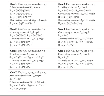
In [10], the authors proposed seven different cases for cell disjoint multiple paths based on the coordinates of the source cell, S, and the coordinates of the destination cell, D, in the 3D-grid. The seven cases cover all the situations where S and D are distinct grid cells. These are shown in Table 1. Under each case,

Table 1. Cell-disjoint routing path definitions for VA-GMPR.

Case 1: If xS ≠ xD, yS ≠ yD, and zS ≠ zD

3 Routing vectors of Lopt length

R1,1 = (−x)*(−y)*(−z)*,

R1,2 = (−y)*(−z)*(−x)*,

R1,3 = (−z)*(−x)*(−y)*

One routing vector of (Lopt + 4) length

R1,4 = +x (−y)* (−z)* (−x)*

Case 2: If xS ≠ xD, yS ≠ yD, and zS = zD

2 routing vectors of Lopt length

R2,1 = (−x)*(−y)*, R2,2 = (−y)*(−x)*

One routing vector of (Lopt + 2) length

R2,4 = z−(−x)*(−y)*z+

One routing vector of (Lopt + 4) length

R2,5 = +x (−y)*+ (−x)*−y

Case 3: If xS ≠ xD, yS = yD, and zS ≠ zD

2 routing vectors of Lopt length

R3,1 = (−x)*(−z)*, R3,2 = (−z)*(−x)*

2 routing vectors of (Lopt + 2) length

R3,3 = y+ (−x)*(−z)*y−,

R3,4 = y− (−x)*(−z)*y+

Case 4: If xS ≠ xD, yS = yD, and zS = zD

One routing vector of Lopt length

R4,1 = (−x)*

3 routing vectors of (Lopt + 2) length

R4,2 = y+ (−x)*y−, R4,3 = y− (−x)*y+,

R4,5 = z− (−x)*z+

Case 5: If xS = xD, yS ≠ yD, and zS ≠ zD

2 routing vectors Lopt length

R5,1 = (−y)* (−z)*, R5,2 = (−z)* (−y)*

2 routing vectors of (Lopt + 2) length

R5,3 = x+ (−y)*(−z)*x−,

R5,4 = x− (−y)*(−z)*x+

Case 6: If xS = xD, yS ≠ yD, and zS = zD

One routing vector of Lopt length

R6,1 = (−y)*

3 routing vectors of (Lopt + 2) length

R6,2 = x+ (−y)*x−, R6,3 = x− (−y)*x+,

R6,5 = z− (−y)*z+

Case 7: If xS = xD, yS = yD, and zS ≠ zD

One routing vector of Lopt length

R7,1 = (−z)*

3 Routing vectors of (Lopt + 2) length

R7,2 = x+ (−z)*x−, R7,3 = x− (−z)*x+,

DOI: 10.4236/wsn.2018.107008 140 Wireless Sensor Network GMPR defines six cell-disjoint paths with optimal or near-optimal path lengths. However, the number of disjoint paths in VA-GMPR is restricted to four in or-der to avoid long paths and eliminate infeasible ones in unor-derwater. Because, it is assumed that all sensor nodes are located within the boundaries of the UWSNs region, and that the sink is at a fixed position on the surface. The modified list of the multiple disjoint routing paths definitions for VA-GMPR are shown in Ta-ble 1, which are obtained from the list of paths defined in [26]. Accordingly, all selected multiple paths in VA-GMPR are characterized with optimal or near-optimal path lengths, Lopt, or (Lopt + 2), respectively, with the exception of two paths which are characterized with (Lopt + 4). Those are R1,4 = +x (−z)* (−y)* + (−x)*−y, and R2,5 = +x(y)*+ (−x)*−y.

Examples of paths considered in VA-GMPR from cases 1, 2, and 3 are: R1,1 = (−x)*(−y)*(−z)*,

R2,2 = (−y)*(−x)* R3,3 = y+ (−x)*(−z)* y−

where, Ri,j refers to routing path j of case i. The path lengths of R1,1, R2,2, and R3,3 are Lopt, Lopt, and Lopt + 2, respectively.

However, there are boundary conditions for the valid paths that must be satis-fied. The invalid paths are determined based on the locations of the source and destination cells, which are dropped from the considered subset of multiple paths. For more details on these boundary conditions see [10].

3.3. The VA-GMPR Protocol

DOI: 10.4236/wsn.2018.107008 141 Wireless Sensor Network starting gateway’s NID of the path’s next hop CID. Besides, if a source sensor node does not have a gateway in its local cell, the source node drops the packet.

When an intermediate gateway receives a data packet, it checks if the sink NID in the data packet header match its own gateway’s NID. If it does, the re-ceiving gateway is the sink and the data packet is delivered. Otherwise, if the node is a gateway, and its CID is matching the next-hop CID in the route path of the data packet header, then this gateway is a forwarding gateway for the re-ceived data packet. Accordingly, the forwarding gateway would determine the next-hop CID in the path, and searches for its NID in the neighboring gateways table, Gw-Table. If there is a valid gateway NID for the next-hop CID, the data packet header fields are updated, and the data packet is forwarded to that next-hop NID gateway. If there is no valid gateway NID entry for the next-hop CID in the neighboring gateway table, then the forwarding gateway would start the void avoidance scheme as described in the next section. The flow chart of the VA-GMPR scheme is shown in Figure 1.

DOI: 10.4236/wsn.2018.107008 142 Wireless Sensor Network

4. The Grid Void Avoidance (GVA) Scheme of VA-GMPR

The geographic routing schemes have been shown to be very suitable for UWSNs, because they do not need the communication overhead to discover and maintain the full path from the source to the destination. However, the charac-teristics of underwater environments make it more difficult for such schemes to cope with void regions [27]. Mainly because the void regions are 3D, which re-quire special treatments than 2D voids in terrestrial networks; and because sen-sor nodes mobility in underwater creates mobile void regions. In a grid-based routing scheme, we define a grid cell as a void/hole cell if that cell does not have any sensor node elected as a gateway. This situation may arise due to the lack of deployed sensor nodes, the relocation of gateway nodes due to water currents, the malfunction of existing gateway nodes due to energy depletion or failure, or due to temporary conditions such as the gateway re-election process. In VA-GMPR, we define a path-dead-end gateway as a gateway along the path whose next-hop cell is a void (hole) cell, and we define a dead-end gateway as a gateway which is closer to the destination than any of its neighboring gateways. In this section, the Grid Void Avoidance (GVA) scheme is described as a me-chanism for handling the void problem in VA-GMPR.

The GVA scheme adopts three techniques for handling holes in search for an alternative path to the sink. These are the hole bypass, the path diversion, and the path backtracking/elimination. These three techniques are applied in this order for the three GVA conditions defined below. The failure of one technique would trigger the application of the next one in sequence as will be elaborated next. The objective of the GVA scheme is to reduce the overhead of handling holes, while being able to enhance the reliability of the routing protocol. That is the reason for applying these techniques in increasing order of their complexity.

4.1. Grid-Based Void Avoidance Conditions

In VA-GMPR, whenever a hole is discovered in the next hop, the path-dead-end gateway would determine the specific situation of the GVA scheme to be applied based on the grid cell location of the current forwarding (i.e., path-dead-end) gateway in the path from the source to the destination. Typically, the location of the void grid cell is on a path segment of the route along one of the directions X, Y, or Z. The GVA scheme identifies three void conditions according to the cur-rent location of a discovered void grid cell and the packet’s progression through the routing path. These are defined as follows:

• _{GVA-Condition 1: Completion of progress on two dimensions towards the}

destination. In this situation, the current node and the sink node have equal values in two of their three coordinates. This void condition can be applied to all routing cases.

• _{GVA-Condition 2: Completion of progress on one dimension toward the}

DOI: 10.4236/wsn.2018.107008 143 Wireless Sensor Network routing case 1, case 2, case 3 and case 5.

• _{GVA-Condition 3: Completion of progress on none of the dimensions}

to-wards the destination. In this situation, none of the coordinate values have completed advancement towards the corresponding coordinates of the desti-nation values. This void condition can be applied to routing case 1 only. All GVA procedures for conditions 1, 2, and 3, are referred to as GVA-C1, GVA-C2, and GVA-C3, respectively. They are applied for handling holes in or-der, such that the failure of one technique would trigger the application of the next one in sequence. The GVA procedures are applied each time a hole cell is discovered on the original or modified path from source to destination. The techniques for handling holes are discussed next.

4.2. Hole Bypass Technique

The hole bypass technique in VA-GMPR handles the hole problem by bypassing a void grid cell through one of the path-dead-end gateway neighboring cells in order to return back to the original path segment. The neighboring gateways are acting as bypassing nodes, and they are referred to as bypass gateways. The sub-set of bypassing neighboring gateways is determined based on the current direc-tion of the path segment toward the sink, and the existence of valid two-hop ga-teway along the path segment. In this work, we define the direction of a path segment for a routing path definition as a unit vector, Pd, in 3D consisting of three components (xd, yd, zd). Since each path segment of a routing path defini-tion is parallel to one of the coordinate axes X, Y, or Z; the direcdefini-tion vectors of the path segments are defined as <±1, 0, 0>, <0, ±1, 0>, or <0, 0, ±1>. Accor-dingly, we characterize the relative position of one-hop, two-hop, and bypass neighbors with respect to a forwarding gateway using the following definitions:

Definition 1:

The relative position of a one-hop neighboring grid cell with respect to a for-warding node (xf, yf, zf), along a routing path segment direction Pd, can be de-termined by a vector V1h = Pd, emanating from the forwarding node along the routing path segment direction toward its neighbor.

Definition 2:

The position of a one-hop neighbor of a forwarding node (xf, yf, zf) is called a pivot node if it is the intersection point of two path segments in the routing path definition.

Definition 3:

The relative position of a two-hop neighboring grid cell with respect to a for-warding node (xf, yf, zf), along a routing path segment direction Pd, can be de-termined by a vector V2h defined as follows:

V2h = V1h + Pd; if the one-hop grid cell is not a pivot node, or V2h = V1h + Pd+1; if the one-hop grid cell is a pivot node

DOI: 10.4236/wsn.2018.107008 144 Wireless Sensor Network For example, if Pd= <0, 1, 0> and Pd+1 = <−1, 0, 0>, then

V1h = <0, 1, 0>

V2h = <0, 2, 0>; if the one-hop grid cell is not a pivot node, or; V2h = <−1, 1, 0>; if the one-hop grid cell is a pivot node.

Since the position of a hole cell is at a one-hop location with respect to a path-dead-end node, (xe, ye, ze), along a path segment direction, we restrict the subset of possible bypass grid cells to eight out of the 26 neighbors, in order not to increase the path length of a path definition. Accordingly, these bypass grid cells are defined as follows.

Definition 4:

The eight bypass neighboring grid cells of a path-dead-end node (xe, ye, ze), that do not increase the path length of a routing path definition, are the eight neighboring grid cells located on the perpendicular plan to the path segment di-rection vector, Pd, and passes through the hole cell.

For example, if Pd = <1, 0, 0> and a path-dead-end node is located at (xe, ye, ze), then the hole cell is located at location (xe + 1, ye, ze), and the subset of eight possible bypass neighboring grid cells are: {(xe+ 1, ye + 1, ze), (xe + 1, ye − 1, ze), (xe + 1, ye, ze + 1), (xe + 1, ye, ze − 1), (xe + 1, ye + 1, ze + 1), (xe + 1, ye + 1, ze − 1), (xe + 1, ye − 1, ze + 1), (xe + 1, ye − 1, ze − 1)}.

Basically, the hole-bypass technique is applied in all GVA procedures. The hole bypass technique requires the existence of a valid two-hop gateway along the routing path direction, otherwise it fails. The confirmation that there is an existing two-hop gateway allows the hole bypass technique to select a valid by-pass gateway from one of the eight byby-passing neighboring gateways. The tech-nique fails if it cannot find a valid bypass gateway in any of the eight bypassing neighboring grid cells. In case a valid bypass gateway is found, the routing path in the packet header would be updated by replacing the next-hop CID by the CID of the bypass gateway, and changing the next hop address to the bypass ga-teway NID, then transmitting the packet.

However, the location of the hole cell at the intersection of two path segments, as a pivot, can appear in GVA conditions 2 and 3, where there is a change in the direction. This situation can be detected from the routing path by testing the path direction from the pivot to the two-hop cell and comparing it with the cur-rent path direction. For example, if the path direction is shifting from <±1, 0, 0> to <0, ±1, 0>, or <0, 0, ±1> then the hole cell is a pivot. If there is a valid two-hop gateway, then the original path is updated by just deleting the CID of the hole cell.

4.3. Path Diversion Technique

DOI: 10.4236/wsn.2018.107008 145 Wireless Sensor Network cells in order to avoid the hole cell. The candidate neighboring gateways consi-dered as starting gateways for the alternative path segments are the same as those considered as bypassing gateways in this work. The technique fails if none of the starting gateways exists. This technique is divided into three cases:

• _{Diversion paths in case of completion of progress on two dimensions.} • _{Diversion paths in case of completion of progress on one dimension.}

• _{Diversion paths in case of no completion of progress on any dimension}

to-wards the destination.

4.3.1. Diversion Paths in Case of Completion of Progress on Two Dimensions

The path diversion technique in this case builds a new path segment to the des-tination, based on the current direction (i.e., X, Y, or Z) of the path segment, such that it is in parallel to the original one and starting from one of the candi-date bypassing gateways. The constructed new path segment replaces the origi-nal one in the forwarded packet. The construction of the parallel path segment to the current one is based on route path R4,1 = (−x)*, R6,1 = (−y)*, or R7,1 = (−z)* in cases 4, 6, or 7, respectively, in Table 1.

4.3.2. Diversion Paths in Case of Completion of Progress on One Dimension

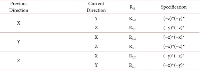
The path diversion technique in this case would build new path segments to the destination based on the current direction, and the previous direction on which progress has been completed. Since progression on the current direction is blocked, due to the discovery of holes on the next one and two hops, the tech-nique would construct new path segments to the destination that allow the path to start progressing on the original next segment first then following it by com-pleting the progression on the original current direction. For example, if the current direction is along the X-axis and the previous direction of the path was on the Y-axis, then the new path segments are constructed to have the next seg-ment on the Z-axis and the final one on the X-axis. The construction of the di-version path in this case follows the cell-disjoint routing vectors of cases 2, 3, and 5 in Table 1. The specifications of the diversion paths are summarized in Table 2. The starting gateway for these diversion paths would be one of the neighboring cells that satisfy the corresponding route vector in Table 2.

Table 2. Definitions of the diversion paths.

Previous

Direction Direction Current Ri,j Specification

X Y R5,2 (−z)*(−y)* Z R5,1 (−y)*(−z)*

Y X R3,2 (−z)*(−x)* Z R3,1 (−x)*(−z)*

DOI: 10.4236/wsn.2018.107008 146 Wireless Sensor Network

4.3.3. Diversion Paths in Case of No Completion of Progress on Any Dimension towards the Destination

In this case we determine a starting gateway with respect to the current path-dead-end gateway based on the current direction of the path segment. A new route starting from one of the bypass gateways to the destination will be generated as follows:

• _{In case of X-direction, if the starting gateway exists in the Y-direction, then}

the new route segment will be computed in a similar manner to route 2 of the routing case 1 (R1,2 = (−y)*(−z)*(−x)*). Otherwise, if the starting gateway ex-ists in the Z-direction, then the new route segment will be computed in a similar manner to route 3 of the routing case 1 (R1,3 = (−z)*(−x)*(−y)*). Oth-erwise, the method is terminated unsuccessfully.

• _{In case of Y-direction, if the starting gateway exists in the X-direction, then}

the new route segment will be computed in a similar manner to route 1 of the routing case 1 (R1,1 = (−x)*(−y)*(−z)*). Otherwise, if the starting gateway ex-ists in the Z-direction, then the new route segment will be computed in a similar manner to route 3 of the routing case 1 (R1,3). Otherwise, the method is terminated unsuccessfully.

• _{In case of Z-direction, if the starting gateway exists in the X-direction, then}

the new route segment will be computed in a similar manner to route 1 of the routing case 1 (R1,1). Otherwise, if the starting gateway exists in the Y-direction, then the new route segment will be computed in a similar manner to route 2 of the routing case 1 (R1,2). Otherwise, the method is terminated unsuccessfully. Then, the new remaining path segment grid coordinates will be mapped to CIDs, and the original remaining path segments in the packet header will be re-placed by the new diversion path accordingly.

4.4. Path Backtracking/Elimination Technique

This technique is applied when the path diversion method cannot handle the problem of the hole. In this situation the path-dead-end gateway is a dead-end gateway. It would generate a negative acknowledgment packet which contains the original path in reverse order. The packet is sent on a backward path toward the source gateway in search for an alternative path at any gateway on the path back to the source, until either a new path is found, or the negative acknowl-edgment packet reaches the source gateway. When a negative acknowlacknowl-edgment packet arrives at the source gateway, it would mark this path to the destination as invalid and selects another path from the set of alternative disjoint valid paths to the destination. This approach follows exactly the approach of EMGGR pro-tocol for handling the hole problem, where it is the only approach applied for handling holes.

5. Simulation and Performance Evaluation

DOI: 10.4236/wsn.2018.107008 147 Wireless Sensor Network protocol for UWSNs compared to the Energy-efficient Multipath Grid-based Geographic Routing protocol (EMGGR). The section includes the specifications of the simulation settings that are applied in the simulation experiments in this research, followed by the definitions of the performance metrics used to com-pare different routing protocols. Finally, the simulation results are presented, discussed and analyzed.

5.1. Simulation Settings

All simulations are performed using the underwater sensor network simulation package called Aqua-Sim [28]. Aqua-Sim is based on NS-2 network simulator tools. It effectively simulates the underwater acoustic channels and supports three-dimensional network deployment. We use the broadcast MAC protocol. In this MAC protocol, when a node has a packet to send, it first senses the channel. If the channel is free, it broadcasts the packet. Otherwise, it backs off. The packet will be dropped if the node backs off four times. In all the simulation experi-ments described in this section, sensor nodes were randomly deployed in a space of 300 m × 300 m × 300 m. Each simulation run lasted for 1000 seconds. The results from the first 150 seconds and the last 100 seconds were discarded to mi-nimize the warm-up effect. Each simulated result was obtained from an average of 30 runs. In each run, 25 sources were selected randomly. A more comprehen-sive list of simulation parameters is shown in Table 3.

Table 3. Simulation parameters.

Parameter Description Simulator Aqua-Sim Routing Protocols VA-GMPR, EMGGR

Topology size (300 × 300 × 300) m3

Interface Queue (type & length) Priority Queue , 50 packets MAC type Broadcast MAC Traffic Type Exponential distribution

Bandwidth 50 kbps Mobility Model 2-D random-walk Simulation time 1000 sec. Transmission range (R) 180 m

Initial energy 10000 J Cost of transmission 2.0 W

Cost of reception 0.75 W Idle power 0.01 W Energy threshold 20 J Cell side (d), and grid size (k × k) 50 m, 6 × 6

DOI: 10.4236/wsn.2018.107008 148 Wireless Sensor Network

5.2. Performance Metrics and Operating Conditions

In this work, we have focused on three performance metrics for comparisons between VA-GMPR and EMGGR protocols. These are:

• _{Packet Delivery Ratio (PDR): Is defined as the ratio of the total number of}

packets received by the destination (i.e. sink) to the total number of packets transmitted by all nodes.

• _{Average End to End Delay: This is the average duration taken by a data}

pack-et starting from the time it is transmitted by the source gateway to the time it is being received by the sink.

• _{Energy Consumption: The total energy consumed by all nodes during the}

simulation. It includes the transmission power, the reception power and the idling power consumed by all nodes.

The above performance metrics have been assessed under different operating conditions and scenarios. These are:

• Network Density: In this work, the impact of network density has been as-sessed by varying the number of nodes in the network.

• _{Traffic Load: The impact of traffic load on the protocol performance has}

been assessed by varying the generation rate of the data packets.

• _{Node Mobility: Since underwater nodes are assumed to move with water}

currents, we have studied the impact of node mobility on the performance me-trics mentioned above by varying the maximum speed of the sensor nodes.

5.3. Simulation Results and Analysis

In all simulation experiments, we compare the performance of VA-GMPR with respect to EMGGR using 95% confidence intervals. 25 randomly selected sources inject traffic into the network. The average of the 30 batch runs along with the error bars are presented in the plotted results. The results of the simulation ex-periments for the impact of the network density, traffic load and node mobility are presented next.

5.3.1. Impact of Network Density

DOI: 10.4236/wsn.2018.107008 149 Wireless Sensor Network

Figure 2. Effect of network density with mobile nodes on the PDR.

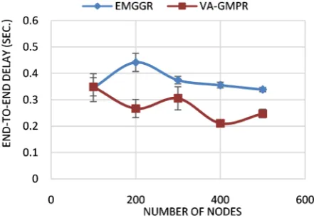
Figure 3. Effect of network density with mobile nodes on the average end-to-end delay.

the VA-GMPR protocol shows better average end-to-end delay than the EMGGR protocol by about 25% on average. This can be attributed to the ability of the VA-GMPR protocol to bypass or reconstruct an alternative path to the destination base on using the GVA scheme. Accordingly, it is able to deliver packets faster than the EMGGR protocol as the density of nodes increases. The impact of network density on the total energy consumption is shown in Figure 4. The two protocols exhibit a similar energy consumption trend with increasing number of nodes. The total energy consumption of EMGGR and VA-GMPR protocols increases with increasing the number of nodes, with VA-GMPR having higher energy consumption than EMGGR by about 21% on average. The overhead of periodic control messages exchanged for maintaining the

GW-Table in each gateway has a negative influence on the energy consumption

of VA-GMPR.

5.3.2. Impact of Traffic Load

DOI: 10.4236/wsn.2018.107008 150 Wireless Sensor Network Figure 5 shows the packet delivery ratio trend against the packet generation rate. It decreases with the increase in the packet generation rate in both VA-GMPR and EMGGR. By increasing the packet generation rate, more packets are propa-gated in the network and hence more packets get dropped due to collision. However, VA-GMPR outperforms EMGGR under all traffic rates. This is mainly due to the availability of the disjoint paths and its ability to deal with holes.

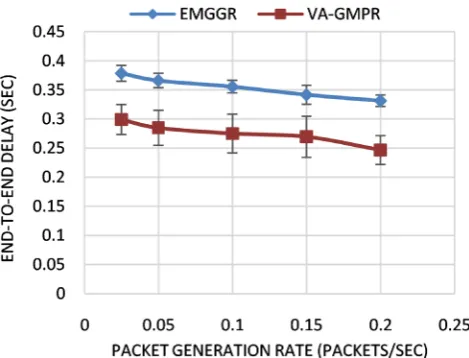
The impact of traffic load on the average end-to-end delay is shown in Figure 6. The figure illustrates that the two protocols exhibit similar trends of average end-to-end delay: as the packet generation rate increases, the average end-to-end delay decreases. The change in the average end-to-end delay is insignificant, be-cause packets are routed from source to destination on multiple paths of close path lengths. However, there is a significant advantage for VA-GMPR over EMGGR in regard to end-to-end delay. According to these simulation scenarios, the VA-GMPR protocol outperforms EMGGR in PDR and end-to-end delay with about 7.5%, and 22.5% on average, respectively. In regard to the impact of

Figure 4. Effect of network density with mobile nodes on the energy consumption.

DOI: 10.4236/wsn.2018.107008 151 Wireless Sensor Network

Figure 6. Effect of traffic load on the average end-to-end delay.

traffic load on the total energy consumption, Figure 7 shows that the energy consumption increases as the traffic load increases in both protocols. But, VA-GMPR protocol shows higher energy consumption compared to EMGGR by about 33% on average, due to the increase of the number of control packets, with the exception of the case of 0.2 packets/sec traffic. In general, the difference in energy consumption between the two protocols decreases with increasing traffic load, which with the accompanied difference in end-to-end delay, implies that EMGGR protocol has high overhead due to its inflexibility in handling holes.

5.3.3. Impact of Node Mobility

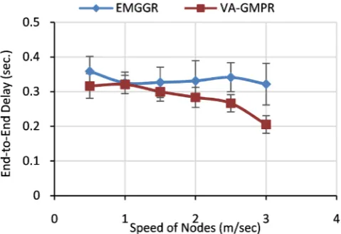
The impact of node mobility is assessed by varying the maximum speed of the nodes from 0.5 m/s to 3.0 m/s, while the minimum speed is fixed to 0.0 m/s. The number of nodes used in this set of simulation experiments is 400 nodes and are deployed randomly in the network. The mean of the exponential distribution of the packet generation rate is set to 0.1 packets per second. Figure 8 shows a common trend of the effect of node mobility on the packet delivery ratio for both VA-GMPR and EMGGR. With increasing the maximum speed of the nodes, the packet delivery ratio is decreasing steadily. This drop in the packet delivery ratio can be attributed to the short period that the gateways may stay in the same cells, which would cause the election process to start over again. How-ever, VA-GMPR outperforms EMGGR in terms of packet delivery by about 24%, because of its ability to handle the existence of holes due to mobility through the hole bypass method or the path diversion method.

DOI: 10.4236/wsn.2018.107008 152 Wireless Sensor Network paths in the EMGGR protocol, because of using backtracking for handling holes. The decline in the average end-to-end delay in VA-GMPR is about 15%, and it is attributed to using the GVA scheme, which gives flexibility to overcome the ef-fect of gateways re-election.

Figure 7. Impact of traffic load on the energy consumption.

Figure 8. Effect of node mobility on the PDR.

DOI: 10.4236/wsn.2018.107008 153 Wireless Sensor Network Figure 10 shows the impact of node mobility on the total energy consump-tion. The figure shows that as the speed of nodes increases, the total energy con-sumed in both VA-GMPR and EMGGR decreases, because of the dynamic crea-tion of holes in the network that results in reducing the rate of packets delivered. However, the energy consumption of VA-GMPA is still higher than EMGGR by about 46%.This can be attributed to the frequent loss of gateways due to the movement of nodes, which has an effect on the frequent application of the GVA scheme. Basically, with each disappearance of a gateway, a temporary hole may be created until the re-election process creates another gateway, or a permanent hole is generated. In addition, the overhead of control messages exchanged for obtaining two-hop neighboring gateways to maintain the GW-Table has an ef-fect on increasing the energy consumption of the VA-GMPR compared to the EMGGR.

6. Conclusion and Future Work

In this work, we have proposed a geographic routing protocol, called VA-GMPR, for UWSNs based on a 3D virtual grid structure. The VA-GMPR performs mul-tipath construction using optimal or near-optimal cell-disjoint paths to enhance network reliability and load balancing. In order to tackle the hole problem, a void avoidance mechanism, called GVA, is adopted as a solution through three techniques. The GVA techniques are applied in increasing order of complexity according to the extent of the void region, and these are the hole bypass, the path diversion, and the path backtracking. We have evaluated the performance of the proposed VA-GMPR protocol by simulation and compared the results to a re-cently proposed grid-based routing protocol, called EMGGR. The simulation results show the effectiveness of VA-GMPR performance with respect to EMGGR, though with higher energy consumption.

However, the VA-GMPR protocol has limitations due to applying the k-ary n-cube approach of interconnection networks by constructing routing paths

DOI: 10.4236/wsn.2018.107008 154 Wireless Sensor Network based on the existence of 6 one-hop neighbors, although the connectivity is 26 and can be extended to 32 by including some two-hop neighbors in a wireless network. An extension work of the protocol can be applied to allow routes mak-ing use of the available high connectivity in 3D. Besides, the protocol relies on the election of one gateway in each cell and the existence of one sink. The relia-bility of the protocol can be enhanced in future work by improving the gateway election process to include more than one gateway in each cell, and considering an architecture that includes multiple sinks. The high energy consumption of the protocol is a drawback, and it can be also addressed in future work by eliminat-ing or reduceliminat-ing the need for control messages to determine 2-hop neighbors, or by implementing the protocol using a distributed routing scheme rather than source routing to reduce the size of the packet header.

Acknowledgements

The authors gratefully acknowledge the support provided by The Research Council (TRC) of the Sultanate of Oman, under the research grant number RC/SCI/COMP/15/02.

Conflicts of Interest

The authors declare no conflicts of interest regarding the publication of this pa-per.

References

[1] SavetheSea.org Website (2018). http://www.savethesea.org/STS%20ocean_facts.htm [2] AUV Laboratory at MIT Sea Grant (2018).

http://auvlab.mit.edu/publications.html

[3] Akyildiz, F., Melodia, T. and Pompili, D. (2005) Underwater Acoustic Sensor Net-works: Research Challenges. Ad Hoc Networks, 3, 257-279.

https://doi.org/10.1016/j.adhoc.2005.01.004

[4] Manjula, B. and Manvi, S. (2011) Issues in Underwater Acoustic Sensor Networks. International Journal of Computer and Electrical Engineering, 3, 1793-8163. [5] Ayaz, M., Baig, I., Abdullah, A. and Faye, I. (2011) A Survey on Routing Techniques

in Underwater Wireless Sensor Networks. Journal of Network and Computer Ap-plications, 34, 1908-1927. https://doi.org/10.1016/j.jnca.2011.06.009

[6] Jiang, Z.H. (2008) Underwater Acoustic Networks-Issues and Solutions. Interna-tional Journal of Intelligent Control and Systems, 13, 152-161.

[7] Akkaya, K. and Younis, M. (2005) A Survey on Routing Protocols for Wireless Sensor Networks. Ad Hoc Networks, 3, 325-349.

https://doi.org/10.1016/j.adhoc.2003.09.010

[8] Erol-Kantarci, M., Mouftah, H. and Oktug, S. (2011) A Survey of Architectures and Localization Techniques for Underwater Acoustic Sensor Networks. IEEE Commu-nications Surveys & Tutorials, 13, 487-502.

https://doi.org/10.1109/SURV.2011.020211.00035

DOI: 10.4236/wsn.2018.107008 155 Wireless Sensor Network Swarm Optimization Algorithms. Sensors, 16, 212.

https://doi.org/10.3390/s16020212

[10] Day, K., Harous, S., Touzene, A. and Arafeh, B. (2011) A Reliable Multipath Routing Protocol for Mobile Ad-Hoc Networks: Adapting Techniques From Inter-connection Networks. Journal of Interconnection Networks, 12, 19-54.

https://doi.org/10.1142/S0219265911002836

[11] Al Salti, F., Alzeidi, N. and Arafeh, B. (2017) EMGGR: An Energy-Efficient Multi-path Grid-Based Geographic Routing Protocol for Underwater Wireless Sensor Network. Wireless Networks, 23, 1301-1314.

https://doi.org/10.1007/s11276-016-1224-0

[12] Cui, J.-H., Lao, L. and Xie, P. (2006) VBF: Vector-Based Forwarding Protocol for Underwater Sensor Networks. Proceedings of IFIP Networking’06, Coimbra, 15-19 May 2006, 1216-1221.

[13] Nicolaou, N., See, A., Xie, P., Cui, J.-H. and Maggiorini, D. (2007) Improving the Robustness of Location-Based Routing for Under-Water Sensor Networks. IEEE Proceedings OCEANS 2007-Europe, Aberdeen, 18-20 June 2007, 1-6.

[14] Yu, H., Yao, N. and Liu, J. (2015) An Adaptive Routing Protocol in Underwater Sparse Acoustic Sensor Networks. Ad Hoc Networks, 34, 121-143.

https://doi.org/10.1016/j.adhoc.2014.09.016

[15] Xie, P., Zhou, Z., Peng, Z. Cui, J.-H. and Shi, Z. (2009) Void Avoidance in Three-Dimensional Mobile Underwater Sensor Networks. Proceedings of 4th Int. Conference on Wireless Algorithms Systems and Applications, Boston, 16-18 Au-gust 2009, 305-314. https://doi.org/10.1007/978-3-642-03417-6_30

[16] Jornet, J.M., Stojanovic, M. and Zorzi, M. (2008) Focused Beam Routing Protocol for Underwater Acoustic Networks. Proceedings of the 3rd ACM International Workshop on Underwater Networks, San Francisco, 15-15 September 2008, 75-82. [17] Shin, D., Hwang, D. and Kim, D. (2012) DFR: An Efficient Directional

Flood-ing-Based Routing Protocol in Underwater Sensor Networks. Wireless Communi-cations and Mobile Computing, 12, 1517-1527.https://doi.org/10.1002/wcm.1079 [18] Al-Karaki, J. and Kamal, A. (2004) Routing Techniques in Wireless Sensor

Net-works: A Survey. IEEE Wireless Communication, 11, 6-28. https://doi.org/10.1109/MWC.2004.1368893

[19] Liao, W.-H., Sheu, J.-P. and Tseng, Y.-C. (2001) GRID: A Fully Location-Aware Routing Protocol for Mobile Ad Hoc Networks. Telecommunication Systems, 18, 37-60.https://doi.org/10.1023/A:1016735301732

[20] Wu, Z., Song, H., Jiang, S. and Xu, X. (2007) Energy-Aware Grid Multipath Routing Protocol in MANET. 1st Asia International Conference on Modelling & Simulation, Phuket, 27-30 March 2007, 36-41.https://doi.org/10.1109/AMS.2007.36

[21] Banimelhem, O. and Khasawneh, S. (2012) GMCAR: Grid-Based Multipath with Congestion Avoidance Routing Protocol in Wireless Sensor Networks. Ad Hoc Networks, 10, 1346-1361.https://doi.org/10.1016/j.adhoc.2012.03.015

[22] Chi, Y.-P. and Chang, H.-P. (2013) An Energy-Aware Grid-Based Routing Scheme for Wireless Sensor Networks. Telecommunication Systems, 54, 405-415.

https://link.springer.com/article/10.1007/s11235-013-9742-x

[23] Arafeh, B., Day, K., Touzene, A. and Alzeidi, N. (2014) Multipath Grid-Based Enabled Geographic Routing for Wireless Sensor Networks. Wireless Sensor Net-work, 6, 265-280.https://doi.org/10.4236/wsn.2014.612026

DOI: 10.4236/wsn.2018.107008 156 Wireless Sensor Network Grid Based MANET Routing Protocol with Simple Cell-Head Election. Internation-al JournInternation-al of Wireless and Mobile Computing, 7, 159-170.

https://doi.org/10.1504/IJWMC.2014.059722

[25] Day, K., Touzene, A., Arafeh, B. and Alzeidi, N. (2017) GARP: A Highly Reliable Grid Based Adaptive Routing Protocol for Underwater Wireless Sensor Networks. International Journal of Computer Networks & Communications,9, 71-82. https://doi.org/10.5121/ijcnc.2017.9506

[26] Al-Subhi, T. (2016) Void Avoidance Grid Multipath Position-Based Routing Pro-tocol for Underwater Wireless Sensor Networks. M.Sc. Thesis, Department of Computer Science, Sultan Qaboos University, Muscat.

[27] Ghoreyshi, S.M., Shahrabi, A. and Boutaleb, T. (2017) Void-Handling Techniques for Routing Protocols in Underwater Sensor Networks: Survey and Challenges. IEEE Communications Surveys & Tutorials, 19, 800-827.

https://doi.org/10.1109/COMST.2017.2657881