Robust Quantization for General Similarity Search

(1)

Robust Quantization for General Similarity Search

Yuchen Guo

∗

, Guiguang Ding

∗

, and Jungong Han

Abstract—The recent years have witnessed the emerging of vec-tor quantization (VQ) techniques for efficient similarity search. VQ partitions the feature space into a set of codewords and encodes data points as integer indices using the codewords. Then the distance between data points can be efficiently approximated by simple memory lookup operations. By the compact quantiza-tion, the storage cost and searching complexity are significantly reduced, thereby facilitating efficient large-scale similarity search. However, the performance of several celebrated VQ approaches degrades significantly when dealing with noisy data. Additionally, it can barely facilitate a wide range of applications as the distortion measurement only limits to ℓ2 norm. To address the

shortcomings of the squared Euclidean (ℓ2,2 norm) loss function

employed by the VQ approaches, in this paper, we propose a novel robust and general VQ framework, named RGVQ, to enhance both robustness and generalization of VQ approaches. Specifically, aℓp,q-norm loss function is proposed to conduct the

ℓp-norm similarity search, rather than theℓ2 norm search, and

the q-th order loss is used to enhance the robustness. Despite the fact that changing the loss function toℓp,q norm makes VQ approaches more robust and generic, it brings us a challenge that a non-smooth and non-convexorthogonality constrainedℓp,q -norm function has to be minimized. To solve this problem, we propose a novel and efficient optimization scheme and specify it to VQ approaches and theoretically prove its convergence. Extensive experiments on benchmark datasets demonstrate that the proposed RGVQ is better than the original VQ for several approaches, especially when searching similarity in noisy data.

Index Terms—Vector quantization, similarity search, efficiency, large scale, robustness, generalization, optimization, experiment

I. INTRODUCTION

S

IMILARITY search, a.k.a., nearest neighbor (NN) search, is of great importance in various applications, such as data mining [1], machine learning [2], information retrieval [3], and etc. Formally, NN search is defined as follows: given a setSof points in a metric spaceMand a query pointq∈ M, find the closest point in S toq. One straightforward way is to linearly scan S and compute the distance d(q, xi) between q and

any point xi ∈ S. However, when dealing with a large-scale

dataset, linear scanning is time consuming due to the expensive distance computing operations. Therefore, how to perform efficient NN search in large-scale dataset is an important and practical problem, which has drawn considerable research interest from both academia and industry in the past decades.

Yuchen Guo and Guiguang Ding are with the School of Software, Ts-inghua University, Beijing 100084, China. Email: [email protected], [email protected].

Jungong Han is with the School of Computing and Communica-tions, Lancaster University, Lancaster, LA1 4YW, UK. Email: [email protected].

∗_{Yuchen Guo and Guiguang Ding contributed equally to this paper.}

Corresponding author: Guiguang Ding.

This research was supported by the National Natural Science Foundation of China Grant No. 61571269, and the Royal Society Newton Mobility Grant IE150997.

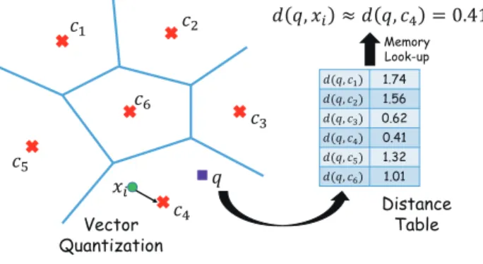
ܿଵ ܿଶ

ܿଷ

ܿସ ܿହ

ܿ଺

Vector Quantization

ݔ௜ ݍ

݀(ݍ,ܿଵ) 1.74

݀(ݍ,ܿ_ଶ) 1.56

݀(ݍ,ܿଷ) 0.62

݀(ݍ,ܿସ) 0.41

݀(ݍ,ܿହ) 1.32

݀(ݍ,ܿ଺) 1.01 Distance

Table

݀ ݍ,ݔ_௜ ൎ ݀ ݍ,ܿ_ସ = 0.41 Memory Look-up

Fig. 1: Illustration of vector quantization based ANN search.

Considering the difficulty of exact NN search for large-scale dataset, approximate NN (ANN) search is regarded as a more practical solution which can simultaneously achieve orders of magnitude speed-ups than exact NN search and near optimal accuracy with proper designs [4]. One paradigm is to utilize the tree structure, such as k-d tree [5]. Theoretically, by recursively bi-partitioning the feature space, tree structure can reduce the frequency of distance computation toO(logn). However, because of thecurse of dimensionality, tree structure may degenerate to sub-linear complexity in high-dimensional spaces since it needs to visit too many branches [6]. Al-ternatively, vector quantization (VQ) emerges recently which is capable of handling high-dimensional data. Different from tree structure that reduces the number of scanned points, the aim of VQ is to speed up the exhausting distance computing. Specifically, VQ partitions the space into a set of codewords, i.e., a codebook C (|C| ≪ |S|), and then quantizes each pointxiinto the codewords. After the quantization, the feature

vector of each point is no longer needed and only an integer index denoting which codeword the point is quantized into is stored. Given a query, its distanced(q, cj)to all codewords can

be pre-computed and stored in a distance table. The distance

(2)

0 1 2 3 4 5 0.4

0.5 0.6 0.7

Noise ratio (%)

Recall@1000

ITQ

(a) SIFT1M,64bits

0 1 2 3 4 5 0.4

0.5 0.6 0.7

Noise ratio (%)

Recall@1000

OPQ

(b) SIFT1M,32bits

0 10 20 30 40 50 1.85

1.9 1.95 2 2.05

#Iterations

Distortion (

×

10

7)

ITQ

(c) SIFT1M,64bits,p= 1

0 10 20 30 40 50 1.4

1.6 1.8 2

#Iterations

Distortion (

×

10

3)

OPQ

(d) SIFT1M,32bits,p= 1

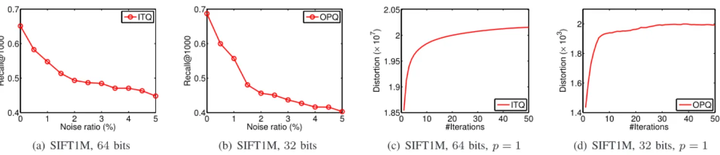
Fig. 2: Traditional VQ approaches perform bad with the noisy data and can not deal with some other similarity measures.

the quantization is performed in each subspace independently, and Additive Quantization (AQ) [13], [14], [15], [16] which constructs several independent codebooks and each point is approximated by summing up the selected codewords from each codebook. As VQ approaches can achieve extreme data compression and support efficient ANN search for large-scale dataset, they have been adopted by many applications, such as image retrieval [17], [18], [19], [20] and many other tasks [21].

A. Problem Statement

The extraordinary performance and widely usage of the VQ approaches motivate as to closely investigate these algorithms. Though specific formulations may have tiny differences, these VQ approaches can be all formulated as a general problem:

min

R,Q,C n X

i=1

kxiR−Q(xi,C)k22, s.t.RR′ =I (1)

where xi ∈Rd is the d-dimensional feature vector, Qis the

quantization function with the codebook C, R ∈ Rd×d _{is a}

rotation matrix which can optimize the quantization [8], [10], [16], andIis the identity matrix. A close look at the objective function reveals that a squaredℓ2loss is applied to measure the

distortion. But unfortunately, this sort of distance measurement comes with certain vulnerabilities. For instance, there are noise and outliers in real-world datasets but the squared loss is sensitive to them because their large distortion will dominate the sum of the squared loss [22], [23], [24], which may markedly degrade the quality of quantization codes. Solving this problem becomes important when we need to search nearest neighbors for data in the wild, such as Flickr images and YouTube videos, as the noises are commonly existed. To verify our observation, we carried out an experiment based on SIFT1M [25] dataset, in which the noise is manually added into the training data and we plot the ANN search performance of two representative VQ approaches, ITQ [8] and OPQ [10], w.r.t. the noise ratio, which is shown in Fig. 2(a) and 2(b) respectively. Obviously, the performance of VQ degrades significantly in the noisy environment, even with only 1% noisy data. Secondly, existing VQ approaches work well for

ℓ2-norm similarity search, i.e.,d(q,xi) =kq−xik2 because

they focus on minimizing ℓ2-norm distortion defined in Eq.

(1). However, when other measurements, such as Manhattan distancedM(q,xi) =kq−xik1[26], are used, their

optimiza-tion objective may fail to well preserve the similarity structure.

In practice, the preferred measure means may need to be defined by users depending on the specific applications, which indicates that a good similarity search algorithm should be generic enough to deal with different distance measurements. Again, to demonstrate this, we plot theℓ1-norm distortion (i.e.,

P

ikxiR−Q(xi,C)k11) w.r.t. the number of iterations of ITQ

and OPQ in Fig. 2(c) and 2(d) respectively. It can be observed that the distortion keeps increasing with more iterations, rather than decreasing, because their optimization algorithms are designed for ℓ2-norm distortion instead of the ℓ1-norm one.

This inevitably leads to less effective quantization function, thereby resulting in worse search performance.

B. Contributions

The two problems mentioned above are important for VQ approaches from both theoretical and practical perspectives, but underestimated by the previous works. This motivates us to develop an improved VQ framework with dual goal to enhance both algorithm robustness and generalization. Recently, several works have demonstrated that theq-th order (q <2, especially

q≤1) ofℓ2loss, i.e.,kxiR−Q(xi,C)kq₂, is less susceptible to

the noise and outliers in data than the squared loss [27], [28]. In addition, according to the triangle inequality, preserving the ℓp-norm distance can be achieved by minimizing theℓp

-norm distortion, i.e., kxiR−Q(xi,C)kp. Therefore, in this

paper, we propose a general VQ framework using a ℓp,q

-norm loss function for learningℓp-norm similarity-preserving

quantization function with more robustness, termed asRGVQ. In summary, this paper makes the following contributions:

• We put forward a newℓp,q-norm loss function for vector

quantization based ANN search. It is robust to noise and outliers by adopting a smallq(e.g.,q≤1) and supports

ℓp-norm (p≤2) similarity search with theℓp-norm loss. • To minimize the obtained orthogonality constrainedℓp,q

-norm function, a novel and efficient iterative optimization algorithm is proposed and its convergence property is theoretically investigated. To our best knowledge, it is the first work that provides the theoretical solution to this challenging non-smooth and non-convex problem.

(3)

TABLE I: Some notations and descriptions in this paper.

Notation Description

n the number of training samples

d the dimension of training samples

C the number of codebooks

k the number of codewords in each codebook

xi the i-th sample

cm

j the j-th codeword in them-th codebook

R a rotation matrix

p,q positive scalars for matrix norm

I the indexing function

• RGVQ is robust to the noise, enabling us to search

sim-ilarity in wild data. Such an framework is favorably de-manded by the applications like Internet image retrieval. Extensive image retrieval experiments on benchmarks collected from the Internet demonstrate the effectiveness.

• Our algorithm is more generic in the sense that multiple

distortion measurements are implemented in one frame-work, allowing us to facilitate a wide range of applica-tions in which various measurements may be requested.

II. PRELIMINARIES ANDRELATEDWORK A. Vector Quantization Approaches

In this paper, we focus on three celebrated VQ approaches, Iterative Quantization (ITQ) [8], [9], (Optimized) Product Quantization (PQ) [10], [11], [12], and Additive Quantization (AQ) [13], [14], [15], [16]. As was mentioned above, these approaches share a general learning objective presented in Eq. (1) but they have different specific formulations and basic ideas. In this section, we will introduce them in details.

ITQ focuses on binary quantization defined as Q(xi,C) =

sign(xiR), wheresign(x) = 1 ifx >0 or−1 otherwise. Its

learning objective is to find the optimal rotation matrix Rto minimize the distortion between the original features and the binary embedding as follows:

min

R OITQ = n X

i=1

kxiR−sign(xiR)k22, s.t. RR′=I (2)

After the binarization, the original distance is approximated by the Hamming distance which is defined as the number of different bits between binary codes (a.k.a., hashcodes), and its computation can be accelerated by either memory look-up or the bit operations (like bit XOR), both of which are efficient. PQ is a k-means clustering like quantization approach. Its basic idea is to cluster the samples into a set of codewords

C ={cj}kj=1 and the distanced(q,xi)can be approximated

by d(q,cI(x_i)) which can be pre-computed and stored in a

distance table. Obviously, increasing the codebook size (i.e.,

k) can partition the space more finely, which improves the distance approximation accuracy. In the extreme case where

k=n, each training sample is quantized to itself such that the distance is precisely approximated. However, whenkis large, computing the distance table, i.e., d(q,cj), becomes a

time-consuming step. Therefore, it is preferable to construct a large

codebook while the extra distance computation is not heavy. To address this issue, PQ proposes to partition the space intoC

orthogonal subspace and the quantization is performed in each subspace independently. Specifically, after the segmentation, each subspace isds=d/C dimension and the final codeword

is constructed by the concatenation of the sub-codeword from each subspace, i.e., cI(x_i)= [c1I1(xi), ...,c

C

IC(xi)] where

cm_j ∈ Cm is a codeword from the m-th subspace. Suppose

there are k codewords for each subspace, i.e.,|Cm| =k, the

total number of codewords in the original space iskC

, which is extremely large. In addition, the distance is approximated by kxi −qk22 ≈

PC

m=1kq

m ₋_cm Im(xi)k

2

2 where qm is

the component of q in the m-th subspace. In this way, the distance table, i.e., d(qm_,_cm

j ), can be computed in each

subspace independently, which reduces the total complexity to

O(C·k· d

C) =O(kd). For good ANN results, PQ minimizes

the distortion between the original features and the codewords:

min R,cm

j ,Im

OPQ=

n X

i=1

kx_iR₋_[c1

I1(xi), ...,

cC

IC(xi)]k 2

2,s.t.RR′=I (3)

whereRis to optimize the quantization, whose effectiveness has been demonstrated by several works [10], [16]. Suppose ˆ

xi =xiRis the rotated data, in PQ, each sub-codebookCm

is learned by k-means clustering in the m-th subspace over

{ˆxi}ni=1and the quantization function is defined asQ(xi,C) =

[c1

I1(xi), ...,c

C

IC(xi)]whereIm(xi) =argminjkˆx

m

i −cmj k22. At

the searching/testing phase, the queryqis also rotated byR. AQ is motivated by the multi-codebook idea of PQ. Differ-ent from PQ which constructs the final codeword by concate-nation, AQ constructs the final codeword by the summation of sub-codewords. In addition, the sub-codeword in PQ isds

dimension while AQ directly constructs sub-codewords in the original space which leads to d-dimensional sub-codeword. Formally, AQ constructsC codebooksCm={cmj }kj=1 where

cm_j ∈Rd. The quantization function is defined asQ(xi,C) =

PC

m=1cmIm(xi). Because we havekq−xik

2

2=kqk22+kxik2₂−

2hq,xii, it is straightforward to approximate the distance by

kq−x_ik2

2 ≈ kqk22+kxik22−2

PC

m=1hq,cmIm(xi)iusing the pre-computed table hq,cm

j i∀m,j. Analogous to PQ, AQ can

also construct kC

codewords in the original space and the complexity to construct the distance table is only O(Ckd). Moreover, AQ attempts to minimize the distortion as follows:

min

R,cm j ,Im

OAQ=

n X

i=1

kxiR−

C X

m=1

cm_I

m(xi)k

2

2, s.t.RR′=I (4)

Theoretically, AQ can be regarded as the generalization of PQ by removing the orthogonal constraints on the sub-codebooks. Because more flexible codeword combination is given, smaller distortion and more accurate quantization can be achieved such that AQ performs better than PQ to some extent [14], [16].

Based on the VQ approaches, the storage cost is markedly compressed and the distance computation is accelerated. For example, in PQ, if we set k = 256 for each sub-codebook, it requires only1 byte (8 bits) to store the index Im(xi)for

(4)

8 gigabytes are required for a 1-billion-size dataset, which can be can be easily handled by only one single machine. During searching, the complexity to compute the distance table is O(Ckd) at most. Since we have Ck ≪ n (in the above example, Ck = 8×256 = 2,048 and n = 1B), the com-plexity is almost ignorable. When computingd(xi,q), onlyC

memory look-up operations andC−1addition operations are required which is far fewer than directly computing d(xi,q)

in an element-wise way, especially for high-dimensional data.

B. Other Related Works

The main focus of this paper is on enhancing the robustness and generalization of existing VQ approaches by introducing theℓp,q-norm loss function to evaluate the quantization

distor-tion. However, we notice several works for some other prob-lems are related to our work [28], [29], [30]. Therefore, it is necessary to introduce them and discuss their difference. Gen-erally, their difference comes from three folds. Firstly, the tasks are different. We focus on vector quantization for efficient and general similarity search including image retrieval, while the others mainly focus on tasks like dictionary learning [28], representation learning [29], and projection learning [30]. In fact, we are the first to introduce a robust loss function and consider the generalization simultaneously in the field of VQ, which motivates us to propose the ℓp,q-norm loss. Moreover,

we specify the general framework to three celebrated VQ approaches, ITQ, PQ, and AQ, which is also very useful in practice. Secondly, the formulations are different. Generally, the ℓ2,q-norm (especiallyℓ2,1-norm) loss is adopted in many

robust learning approaches [28], [29], [30]. But theℓp,q-norm

is more general and complicated than them and it seems that it is difficult to directly apply their optimization algorithm to ℓp,q-norm loss. Some works also consider the ℓp-norm

term. For example, the ℓ1-norm term is considered in sparse

coding [31] and the ℓp-norm is considered in [28]. But it

should be pointed out that our formulation employsℓp-norm

to evaluate the reconstruction distortion while their approaches use it only as a sparsity regularization term for coefficients which element-wise decoupled. Obviously, our formulation is more difficult and general especially when coupling with the

q-th order upon theℓp norm and the orthogonality constraint.

Thirdly, the solutions are different. As stated, our problem is an orthogonality constrainedℓp,q-norm minimization problem.

Unlike some works considering parts of the problem, e.g.,ℓ2,q

-norm minimization is considered in [28], we systematically solve the general problem and provide the theoretical analysis for the solution. In addition, in Section V, we demonstrate that that the optimization algorithm is consistently effective and efficient under different settings.

III. THEPROPOSEDFRAMEWORK A. Overall Objective Function

The first goal of this paper is to enhance the robustness of VQ approaches. In the current framework, squared Euclidean (i.e.,ℓ2,2-norm) loss is adopted. In fact, because of the square

operation, the loss function tends to assign large weight to large-loss samples. However, in practice, the large loss is

often caused by noise and outliers. The loss function, in such a situation, will focus on the noise but fail to capture the intrinsic structure of samples, i.e., it is sensitive to noise, which has been empirically demonstrated in Fig. 2(a) and 2(b). To address this issue, we should reduce the weight of large-loss samples. In this paper, we propose to replace the squared loss by theq-th order loss. It has been demonstrated in several literatures [22], [23], [24], [32] that the loss function is more robust (less sensitive) to the noise and outliers in data in case ofq <2, especiallyq≤1. Motivated by this idea, we reformulate Eq. (1) from squared loss intoq-th order loss as:

min

R,Q,C ORQ= n X

i=1

kxiR−Q(xi,C)kq₂, s.t.RR′ =I (5)

whereq <2. It is not difficult to observe the following fact.

When q >1, the objective prefers to decrease the distortion

of large-loss entries because it is obvious that the largerx(the distortion) is, the larger|xq₋₍_x₋_∆_x₎q_|

(the change in loss) is if ∆xis identical, which indicates the loss is encouraged to fit the noisy data. On the other hand, when q ≤ 1, the situation is different where the loss focuses more on the small-loss entries which are normal data. In this way, we can enhance the robustness of functions by settingq <2, especiallyq≤1. Although theℓ2,q-norm loss function is more robust to the

noise, it is still questionable whether it works well for the other similarity/distance measurements, like Manhattan distance. In fact, just like the results shown in Fig. 2(c) and 2(d), the ℓ2

-norm loss may fail when dealing withℓ1-norm based similarity

search. To address this issue, we firstly revisit one important theoretical building block of VQ, i.e., the triangle inequality:

|kx−ykp− kQ(x)−Q(y)kp| ≤K1kx−y−Q(x) + Q(y)kp

≤K2(kx−Q(x)kp+ky−Q(y)kp) (6)

where kxkp = (Pj|xj|p)

1

p _{is the} ℓ_p_{-norm of a vector,}

K1 = K2 = 1 for normal vector norm (i.e., p > 1) and

they are some constants for quasi-norm (i.e., 0 < p ≤ 1), andQ(x)denotes the quantization result of x. The first term denotes the distance approximation error between the original feature based distance (kx−ykp) and the quantized feature

based distance (kQ(x)−Q(y)kp), in which we expect the error

to be as small as possible, i.e., the distance approximation using the quantized vectors is more accurate. The last term is exactly the distortion caused by the quantization function (kx−Q(x)kp). Obviously, the distortion provides an upper

bound for the distance approximation. Therefore, decreasing the distortion leads to more accurate distance approximation and further results in better ANN performance [8], [10], [15]. Fortunately, based on the triangle inequality, it is straightfor-ward to observe that learning ℓp-norm similarity preserving

quantization function can be achieved by minimizing theℓp

-norm distortion. In the extreme case where the distortion is0 (i.e., Q(x) =x), the distance is perfectly approximated (i.e.,

kx−ykp = kQ(x)−Q(y)kp). Theoretically, existing VQ

(5)

rewrite the loss in Eq. (5) from theℓ2-norm loss to theℓp-norm

loss, leading to the overall objective function of RGVQ:

min

R,Q,C ORG=kXR−Q(X,C)k q p,q =

n X

i=1

kxiR−Q(xi,C)kqp

s.t.RR′ =I (7)

wherekAkp,qdenotes the entrywise (in row) matrixℓp,qnorm

of matrixA. So far, we derive theℓp,q-norm loss function for

RGVQ framework from the original ℓ2,2-norm loss of VQ.

B. Optimization Algorithm

The motivation of changing theℓ2,2-norm loss into theℓp,q

-norm loss is clear and reasonable, which makes VQ more robust to noisy data and generalizable for different distance measurements. However, it is challenging to minimize the ob-tained orthogonality constrainedℓp,q-norm function because it

becomes a non-smooth and non-convex optimization problem when p ≤ 1 or q ≤ 1. Solving this problem is much more difficult than minimizing theℓ2,2-norm in the original VQ, for

which many solutions are available [8], [10], [14]. To solve it, we propose an efficient optimization algorithm shown below. It should be noticed that there are a rotation matrix R, quantization functionQ and the codebookC in the objective function, and it is very difficult, if not impossible, to optimize them as a whole. Therefore, following the traditional VQ framework, we adopt an iterative optimization scheme to update any of them while keeping the others fixed as follows.

Update R. This is the most difficult part in the entire

solution, which is also an important theoretical contribution of this paper. The ℓp,q-norm is neither smooth nor convex,

and meanwhile, the orthogonality constraint limits the feasible set, therefore making the problem more difficult. First, we denote yi = Q(xi,C)as the quantized vector, which is fixed

when updatingR. Then, to solve the problem, we rewrite the complicatedℓp,q-norm loss into a weightedℓ2,2-norm loss as:

min RR′=IO=

n X

i=1

kwi◦(yi−xiR)k22 =kW◦(Y−XR)k2F (8)

whereX= [x1;...;xn]∈Rn×drepresent the original training

vectors, Y = [y1;...;yn] ∈Rn×d are the quantized vectors,

W= [w1;...;wn]∈Rn×d is the weighting matrix,k · kF is

the Frobenius norm of a matrix, and “◦” denotes the element-wise multiplication operation. Specifically, the elements of the weighting matrix in our algorithm are computed as follows:

fi=kyi−xiRkqp−p, gij=|yij−xiR∗j|p−2

wij = (figij)0.5 (9)

Based on the above definition, it is easy to verify that Eq. (8) is numerically equivalent to Eq. (7). Now if we keep W fixed, the problem is transformed into a weighted ℓ2,2-norm

problem. Fortunately, solving this problem is much easier than solving the original as it is smooth and convex. The only challenge left in this problem is to address the orthogonality constraint which limits the feasible set. In this paper, we adopt the framework proposed by Wen et al. [33] which is a gradient-descent based algorithm but takes the orthogonality

constraint into consideration. In particular, we first compute the derivative ofOw.r.t. the variableRas:

G= ∂O

∂R =X

′₍_W_◦_W_◦₍_XR₋_Y₎₎

(10)

In the conventional gradient descent method, we just need to update R along the direction given by the derivative with a tiny step. However, this strategy will violate the orthogonality constraint which moves Rout of the feasible set. Therefore, more operations on the gradient are required to address the orthogonality constraint. Following the framework [33], a skew-symmetric matrix is constructed based onGas below:

A=GR′−RG′ (11)

Having obtainedGandA, the following step is to search the next point using the Crank-Nicolson-like scheme [34], [35]:

Rt+1=Rt−τA(

Rt+1+Rt

2 ) (12)

whereτ is a tiny step size. The solution to the problem is:

Rt+1= (I+τ

2A)

−1₍_I₋τ

2A)Rt (13) The objective function value in Eq. (8) will keep decreasing w.r.t. the updating rule in Eq. (13) until the stationary point is achieved andRt+1 also satisfies the orthogonality constraint.

Please refer to [33] for the detailed proof. We update R by fixingWas we can seeWdepends on R. Therefore, we can update R and W in an iterative manner. This strategy can decrease the loss in Eq. (7), whose proof will be given later.

UpdateQandC. When the rotation matrixRis fixed, we

can update the quantization functionQand the corresponding codebookC. In this paper, we focus on three celebrated VQ approaches, ITQ, PQ, and AQ, which achieve state-of-the-art ANN performance, and therefore we specify our RGVQ framework into these approaches. As they have different formulations and codebook construction methods, the updating rules should be different, each being discussed below. For simplicity, we denote ˆxi=xiR in the following derivation.

ITQ. ITQ focuses on binary quantization and the sign function is adopted, so it does not have a codebookC. Thus, extending it from theℓ2,2normal loss in the original VQ to the

ℓp,q norm loss in RGVQ is the easiest one. Moreover, we can

observe that the quantization in ITQ is element-wise decoupled even with theℓp,q-norm loss. Therefore, the quantized vector

isyij= sign(ˆxij), which is the quantization function for ITQ.

PQ. In the original PQ withℓ2,2-norm loss,it only requires

performing k-means clustering in each subspace to learn each sub-codebookCmand the corresponding function Im. In the

RGVQ framework with the ℓp,q-norm loss, its loss function

for this step is more complicated, which is written as follows:

min

cm j ,Im

ORGPQ=

n X

i=1

(

C X

m=1

ds

X

j=1

(ˆxmij−c m Im(xi)j)

p

)qp ₍₁₄₎

(6)

Algorithm 1 Optimization Algorithm for RGVQ

Input: Training dataX; Parametersp≤2 andq≤p;

Output: Orthogonal matrix R; CodebooksCm;

1: InitializeR=I,ˆxi=xiR;

2: repeat

3: Update weights by Eq. (9);

4: For ITQ: updateyij = sign(xiR∗j);

5: For PQ: solve Eq. (17) for each subspace by Minkowski weighted kmeans clustering [36];

6: For AQ: solve Eq. (19) by sequential residual minimiza-tion [13], [16] for each sub-codebook;

7: Compute quantized vectoryi with currentQ;

8: Update weights by Eq. (9);

9: UpdateRby Eq. (13) and xˆi=xiR;

10: untilConvergence.

11: ReturnRandCm;

loss in one subspace has influence on the decision in the other subspaces. To simplify the problem, we also adopt the weighting method in Eq. (9) and rewrite the loss function as:

min

cm j ,Im

O=

n X

i=1

fi(

C X

m=1

kˆxm_i −cm_I

m(xi)k

p

p) (15)

Obviously, after the transformation, each subspace becomes decoupled. To clarify it, we can rewrite Eq. (15) as follows:

min

cm j ,Im

O=

C X

m=1

Om=

C X

m=1

(

n X

i=1

fikˆxmi −c

m Im(xi)k

p p) (16)

Therefore, in each subspace we solve the problem below:

min

cm j ,Im

Om=

n X

i=1

fikxˆmi −cmIm(xi)k

p

p (17)

which leads to a Minkowski weighted kmeans clustering[36] problem similar to the original kmeans clustering but with

ℓp-norm loss and weighted samples. It can be easily solved in

the EM framework by iteratively updating the indexIm(xi) =

argminjkxˆmi −cmj kand the centerscmj by the simple gradient

descent algorithm. Such a procedure can be performed in each subspace mindependently. In this way, the function value in Eq. (15) is decreased until convergence is achieved, which also decreases the function value ORGPQ in Eq. (14).

AQ. In the RGVQ framework, the objective function to updateQandCof AQ withℓp,q-norm loss is written as below:

min

cm j ,Im

ORGAQ=

n X

i=1

kxˆi−

C X

m=1

cm_I

m(xi)k

q

p (18)

In order to simplify the problem, we also adopt the weighting method mentioned before, which leads to the following loss:

min

cm j ,Im

O=

n X

i=1

fikˆxi−

C X

m=1

cm_I

m(xi)k

p

p (19)

To solve this problem, we adopt the sequential learning scheme [13], [16] which is widely utilized in many opti-mization problems, such as matching pursuit [37], sparse

coding [38], and binary learning [39]. In particular, each sub-codebookCm is optimized to minimize the residual

sequen-tially by fixing the other sub-codebooks. Denote the residual vector as rm

i = ˆxi−P_m′₆=mc m′

I_m′(xi). When the other sub-codebooks are fixed, the problem w.r.t.Cm is reduced to:

min

cm j ,Im

Om=

n X

i=1

fikri−cmIm(xi)k

p

p (20)

which is a Minkowski weighted kmeans clustering, of which the updating rules forcm

j andImare introduced in PQ. In this

way, we can repeat the residual vector computing and sub-codebook updating for each sub-sub-codebooks until convergence.

IV. THEORETICALANALYSIS

A. Convergence Analysis

In the above section, we introduce how to optimize the challengingℓp,q-norm loss defined by Eq. (7) in the specific

situations of ITQ, PQ, and AQ, which is summarized in Algorithm 1. To simplify the complicated problem, we propose a weighting method shown in Eq. (9) and optimize the transformed problems in Eq. (8), (15), and Eq. (19). From the definition of the weights in Eq. (9), it can be observed that the weights are related to the variablesR,Cm, andImwhich are

to be optimized. In our algorithm, we iteratively update the weights and the variables by fixing the other one. However, it is not easy to figure out why decreasing the transformed loss can decrease the original loss in Eq. (7) since they are not strictly equivalent. In this section, we will theoretically and rigourously prove that the loss function in Eq. (7) is non-increasing at each iteration of Algorithm 1, which implies that the algorithm can reach a stationary point of Eq. (7) finally.

At the first of the proof, we introduce the following lemma: Lemma 1: Given anya >0and0< b≤a, for∀x≥0, we have the inequality:axb₋_bxa₊_b₋_a_≤₀_.

Proof 1: Denote c = b/a and f(x) = xc ₋_cx₊_c₋_1.

Apparently, f(1) = 0. Then, we have f′₍_x_{) =} _cxc−1₋_c_,

leading tof′_{(1) = 0. In addition,}_f′′₍_x_{) =}_c₍_c₋₁₎_xc−2_≤₀

whenx≥0because0< c≤1. This impliesf′₍_x₎_≥₀ _∀_x_∈

[0,1]andf′₍_x₎_≤₀_when_{x >}_{1. Therefore,}_f₍_x₎_≤_f_{(1) = 0.}

Finally, we can obtainaf(xa_{) =}_axb₋_bxa₊_b₋_a_≤_0.

Based on Lemma 1, we can prove the following theorem: Theorem 1: The objective functionORG in Eq. (7) is non-increasing under the updating rules for R in Eq. (13), and

CmandImwhich can minimize Eq. (15) and (19).

Proof 2:LetS=Y−XRt,Z=Y−XRt+1, we have:

Ot

RG=

n X

i=1

(

d X

j=1

|sij|p)

q p,Ot+1

RG =

n X

i=1

(

d X

j=1

|zij|p)

q

p ₍₂₁₎

Based on the proof in [33], we know that the updating rule in Eq. (13) can decrease the value ofOin Eq. (8), i.e., we have

X

ij

figijzij2 ≤

X

ij

(7)

Now if we set a = 2,b =p, xwill be |zij|/|sij|. Based on

the Lemma 1 above, we can obtain the following inequalities

2(|zij|

|sij|

)p₋_p₍|zij|

|sij|

)2+p−2≤0

⇒|zij|p−

p

2|sij|

p−2_|_z

ij|2≤ |sij|p− p

2|sij|

p−2_|_s

ij|2

⇒X

ij

fi(|zij|p−

p

2gijz

2

ij)≤ X

ij

fi(|sij|p−

p

2gijs

2

ij)

(23)

Combining inequalities (22) with (23) will bring us

X

i

fikzikpp=

X

ij

fi|zij|p≤

X

ij

fi|sij|p=

X

i

fiksikpp

(24) Denote a=p,b=q, andx=kzikp/ksikp, then we get

p(kzikp

ksikp

)q−q(kzikp

ksikp

)p+q−p≤0

⇒kzikqp−

q

pksik

q−p

p kzikpp≤ ksikqp− q

pksik

q−p p ksikpp

⇒X

i

(kzikqp− q

pfiksik

p p)≤

X

i

(ksikqp− q

pfiksik

p p)

(25)

Again, if we combine inequalities (24) with (25), we obtain

OtRG+1=

X

i

kzikqp≤

X

i

ksikqp=O

t

RG (26)

which meansORGin Eq. (7) is non-increasing w.r.t. Eq. (13). Denote S= Qt₍_X_,_Ct₎₋_XR_,_Z_{= Q}t+1₍_X_,_Ct+1₎₋_XR_.

We can also have Eq. (21). In addition, by minimizing the loss function value in Eq. (15) and (19), we can obtain Eq. (24) directly. Then together with Eq. (25) we obtain Eq. (26), which indicates that ORG in Eq. (7) is non-increasing when we updateCm andIm by minimizing Eq. (15) and (19).

We have the following inequalities with the above proofs:

ORG(Qt,Rt)≥ ORG(Qt+1,Rt)≥ ORG(Qt+1,Rt+1) (27)

which states thatORG is non-increasing with Algorithm 1.

B. Complexity Analysis

Apparently, our optimization is more complicated than that of the original VQ approaches, it is worthwhile to analyze the algorithm complexity. In fact, since VQ approaches are applied to large-scale dataset, we care more about the relationship between the complexity and the training set size n. When updating R, only the gradient computation in Eq. (10) is related to n, whose complexity is O(n). For ITQ, updating the binary codes requires O(n) time. For PQ, we need to solve C sub-problems in each subspace given by Eq. (17). In the originalℓ2,2-norm loss, updatingCmjust needs to compute

the average of samples belonging to the same cluster, which can be achieved in only one step. In our method, we have to adopt the gradient descent algorithm to update cm_j which needs more steps to reach the optimum. Fortunately, we can adopt the mini-batch based stochastic gradient descent (SGD) where a small batch of training samples (e.g., 256), rather than the whole set, are required to compute the gradient in one single step. Although many steps are required, each step only utilizes a small number of samples such that reaching the

TABLE II: The statistics of datasets.

#database #training #query #feature

SIFT1M 1m 100k 10k 128

GIST1M 1m 100k 1k 960

CIFAR-10 50k 50k 10k 512

NUS-WIDE 184k 50k 1,866 500

optimum needs to traverse the whole set for just a few times. In our experiment, we empirically find out that when trained with100k samples and256mini batch, traversing the training set once (i.e., ≈ 400steps) can result in good performance. In fact, we can notice that the mini-batch SGD has achieved great success recently for gradient based optimization, such as deep model training [40], [41]. Wen et al. [42] also demonstrate that the mini-batch SGD works well for kmeans clustering loss. Therefore, training by mini-batch SGD has a comparable complexity to the original kmeans in our case. For AQ, we can also adopt the mini-batch SGD to solve the sub-problem in Eq. (20) whose complexity is O(n). In addition, as will be demonstrated in the experiment section, Algorithm 1 can always converge within about200iterations. In summary,the increase in complexity due to the use of a more complicated optimization is very limited, meaning that the overall complexity of RGVQ is comparable to that of VQ.

V. EXPERIMENT ANDDISCUSSION

A. Datasets

VQ approaches are so general that can be applied to different kinds of features, including features for image [43], [44], video [45], text [46], [47], or sensing data [48], [49]. To better compare our framework with previous VQ approaches, we mainly focus on image features in the experiment below.

(8)

0 1 2 3 4 5 0.1

0.2 0.3 0.4 0.5

Noise ratio (%)

Recall@1000

ITQ+ ITQ

(a) SIFT1M, 32 bits

0 1 2 3 4 5

0.4 0.5 0.6 0.7 0.8

Noise ratio (%)

Recall@1000

ITQ+ ITQ

(b) SIFT1M, 64 bits

0 1 2 3 4 5

0.8 0.83 0.86 0.89 0.92

Noise ratio (%)

Recall@1000

ITQ+ ITQ

(c) SIFT1M, 128 bits

0 1 2 3 4 5

0.5 0.55 0.6 0.65 0.7

Noise ratio (%)

Recall@10000

ITQ+ ITQ

(d) GIST1M, 32 bits

0 1 2 3 4 5

0.65 0.7 0.75 0.8 0.85

Noise ratio (%)

Recall@10000

ITQ+ ITQ

(e) GIST1M, 64 bits

0 1 2 3 4 5

0.74 0.78 0.82 0.86 0.9

Noise ratio (%)

Recall@10000

ITQ+ ITQ

(f) GIST1M, 128 bits

Fig. 3: Performance comparison between ITQ+ and ITQ w.r.t. the noise ratio. We set l= 10for ground truth.

users. The 500-dimensional bag-of-visual-word feature based on SIFT is utilized for image representation. 1% (1,866) images are used as the queries and the other as the database. From the construction methods of these real-world datasets (search engine returned images or user uploaded and annotated images), we can see they are very noisy, making them ideal benchmarks for testing the robustness of various approaches. The statistics of the datasets are summarized in TABLE II.

B. Settings

Since the primary purpose of this paper is to enhance the robustness and the generalization of existing state-of-the-art VQ approaches, we therefore consider three representa-tive approaches, Iterarepresenta-tive Quantization (ITQ) [8], (Optimized) Product Quantization (PQ) [10], [12], and Additive Quan-tization (AQ) [13], [14], [15]. Specifically, we extend the original approaches from theℓ2,2-norm based VQ framework

into the proposed ℓp,q-norm based RGVQ framework and

then optimize them based on Algorithm 1. When no further statement is given and no ambiguity is triggered, we setp= 2 and q= 1 for most experiment scenarios and we denote the enhanced versions as ITQ+, OPQ+, and AQ+ respectively.

For each sample, we can adopt VQ or RGVQ approaches to quantize it into a fixed-length codes, whose length is denoted as L. When constructing the codes, the below settings are adopted. For ITQ which focuses on learning binary hashcodes, following [8], the original sample is firstly projected into a

L-dimensional space by PCA and the rotation matrix R ∈

RL×L is learned in the L-dimensional space. Then we use the sign function on the rotated data to get the hashcodes and the distance between a query and a sample is given by the Hamming distance (the number of different bits). For PQ and AQ, following [10], [14] the size of each sub-codebook is set as k = 256 such that the integer index Im(xi) needs

exact 1 byte (8 bits). Therefore, to learn 64-bit codes, we should construct C = 64/8 = 8 sub-codebooks. Moreover, we adopt the asymmetric distance computation for computing the distance as we introduced in the previous part of this paper. For all approaches, including both VQ and RGVQ, iterative optimization algorithms are adopted for learning quantization models. As suggested by the original literatures [10], [14], [21], their learning procedures can converge with 200 itera-tions. In the upcoming parts, we will show that RGVQ can also converge fast. Therefore, for all VQ and RGVQ approaches, the maximum number of iterations is consistently set to200.

C. Robustness Study

We firstly investigate the robustness of RGVQ against the noise and outliers. Specifically, we adopt the ANN search task using the SIFT1M and GIST1M datasets. To better investigate this property we have manually added some noise to the training data. In particular, each dimension of each manually added noisy point is sampled from 100× N(0,1) whereN

denotes a Gaussian distribution. Obviously, the distribution of noisy data is different from the that of the original data. A robust algorithm should pay more attention to the normal data. To understand the boundary of the algorithm, we continuously change the noise ratio (NR: the ratio between the manually added noise points and the original points), and evaluate the

ℓ2-norm similarity search performance of different approaches.

Following the settings in [10], [15], [21], we use Recall@R

(9)

0 1 2 3 4 5 0.1

0.2 0.3 0.4 0.5

Noise ratio (%)

Recall@1000

OPQ+ OPQ

(a) SIFT1M, 16 bits

0 1 2 3 4 5

0.4 0.5 0.6 0.7 0.8

Noise ratio (%)

Recall@1000

OPQ+ OPQ

(b) SIFT1M, 32 bits

0 1 2 3 4 5

0.75 0.8 0.85 0.9 0.95

Noise ratio (%)

Recall@1000

OPQ+ OPQ

(c) SIFT1M, 64 bits

0 1 2 3 4 5

0.4 0.5 0.6 0.7 0.8

Noise ratio (%)

Recall@10000

OPQ+ OPQ

(d) GIST1M, 16 bits

0 1 2 3 4 5

0.5 0.6 0.7 0.8 0.9

Noise ratio (%)

Recall@10000

OPQ+ OPQ

(e) GIST1M, 32 bits

0 1 2 3 4 5

0.6 0.7 0.8 0.9 1

Noise ratio (%)

Recall@10000

OPQ+ OPQ

(f) GIST1M, 64 bits

Fig. 4: Performance comparison between OPQ+ and OPQ w.r.t. the noise ratio. We set l= 100for ground truth.

0 1 2 3 4 5

0.1 0.2 0.3 0.4 0.5

Noise ratio (%)

Recall@1000

AQ+ AQ

(a) SIFT1M, 16 bits

0 1 2 3 4 5

0.4 0.5 0.6 0.7 0.8

Noise ratio (%)

Recall@1000

AQ+ AQ

(b) SIFT1M, 32 bits

0 1 2 3 4 5

0.76 0.82 0.88 0.94 1

Noise ratio (%)

Recall@1000

AQ+ AQ

(c) SIFT1M, 64 bits

0 1 2 3 4 5

0.4 0.5 0.6 0.7 0.8

Noise ratio (%)

Recall@10000

AQ+ AQ

(d) GIST1M, 16 bits

0 1 2 3 4 5

0.6 0.7 0.8 0.9 1

Noise ratio (%)

Recall@10000

AQ+ AQ

(e) GIST1M, 32 bits

0 1 2 3 4 5

0.6 0.7 0.8 0.9 1

Noise ratio (%)

Recall@10000

AQ+ AQ

(f) GIST1M, 64 bits

Fig. 5: Performance comparison between AQ+ and AQ w.r.t. the noise ratio. We setl= 100for ground truth.

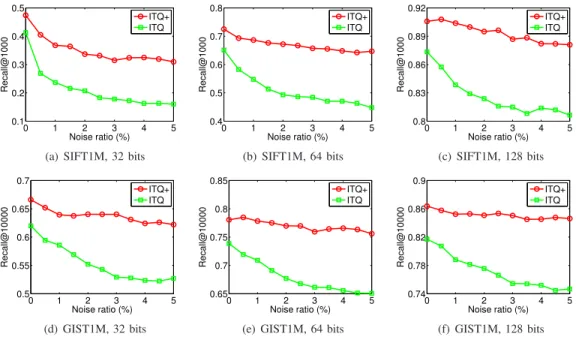
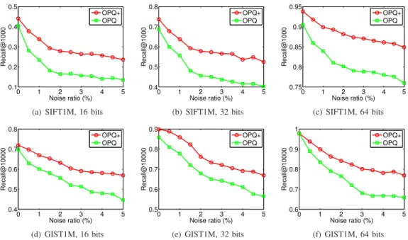
The comparison between RGVQ (ITQ+, OPQ+, and AQ+) and VQ (ITQ, OPQ, and AQ) under different code lengths and noise ratios is shown in Fig. 3, 4, and 5. It can be observed that RGVQ is better than VQ at all situations, including different approaches, code lengths, and noise ra-tios, in terms of the Recall. On average, ITQ+, OPQ+ and AQ+ have improved the recall over ITQ, OPQ, and AQ by 12.2%, 10.8%, and9.85% when NR= 5%, demonstrating that RGVQ withℓp,q-norm (q= 1) loss is indeed more robust

to the noise than the original VQ with squared loss. Moreover, it is worthwhile to point out that the results actually reveal the following properties of the proposed RGVQ framework.

Firstly, RGVQ performs observably better than VQ in most

(10)

8 16 32 64 128 0.18

0.2 0.22 0.24

Code length (bits)

mean Average Precision

ITQ+ ITQ OPQ+ OPQ AQ+ AQ

(a) mean Average Precision

0 0.5 1 0.1

0.15 0.2 0.25 0.3 0.35

Recall

Precision

(b) Precision-recall curve, 16 bits

0 0.5 1 0.1

0.2 0.3 0.4

Recall

Precision

(c) Precision-recall curve, 64 bits

Fig. 6: Performance comparison between RGVQ and VQ on CIFAR-10.

8 16 32 64 128

0.38 0.4 0.42 0.44

Code length (bits)

(a) mean Average Precision

0 0.5 1 0.34

0.36 0.38 0.4 0.42 0.44 0.46

Recall

Precision

(b) Precision-recall curve, 16 bits

0 0.5 1 0.34

0.38 0.42 0.46 0.5

Recall

Precision

(c) Precision-recall curve, 64 bits

Fig. 7: Performance comparison between RGVQ and VQ on NUS-WIDE.

similarity search performance of all VQ approaches degrades rapidly. This phenomenon once again demonstrates that VQ is sensitive to noise and outliers in data because of the squared loss, as we have mentioned before. On the contrary, RGVQ approaches show relatively more stable performance in most cases when we increase NR. More importantly, it can be seen that the performance gap between the corresponding ap-proaches from RGVQ framework and VQ framework becomes even larger when increasing NR. This again demonstrates the superior robustness of the proposed RGVQ against the noise. Moreover, it is observed that ITQ+ is more robust than OPQ+ and AQ+ since the performance drop of ITQ+ when NR raises from0to5%is less significant. One possible reason is that ITQ+ focuses on binary quantization while OPQ+ and AQ+ adopt real-value quantization. As we will show later, ITQ+ has larger distortion because the binary quantization is not that flexible. In this case, the influence of large-distortion entries is relatively smaller in ITQ+ as the majority of entries has large distortion to some extent. Moreover, as OPQ+ and AQ+ have better performance at first, it is more likely that their performance drops more significantly.

D. Image Retrieval Results

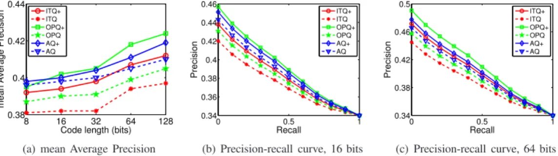
From the application perspective, the robustness of RGVQ enables us to search similarity in wild data such as Internet images. To demonstrate the superiority of RGVQ over VQ, we adopt two widely used image benchmark datasets collected from Web, CIFAR-10 and NUS-WIDE, for the image retrieval task. In particular, in this task, the true positives for each query are defined as the images in the database which share at least one semantic labels/concepts with the query, following [8], [17], [55]. To evaluate the performance, we adopt the

Precision-recall curve as the metric, which reflects the pre-cision (the ratio between the number of true positives and that of retrieved images) at different recall levels. Generally, a higher curve indicates that the true positives have higher ranks which is desired for image retrieval task. Moreover, mean Average Precision (mAP) is also utilized as a numeric evaluation metric. It is defined as the area under the Precision-recall curve and a larger value stands for a better performance.

The results of RGVQ approaches and VQ approaches on CIFAR-10 and NUS-WIDE are presented in Fig. 6 and Fig. 7 respectively. It can be seen that RGVQ consistently outperforms VQ with observable margins with different code length on two datasets. In fact, the real-world image sets are always noisy. Unfortunately, existing approaches fail to consider the influence of noise data. As we have analyzed around Eq. (5), whenqis large, the learning procedure prefers to decrease the loss of large-distortion entries, while it focuses more on the small-distortion entries when q is small. In the VQ approaches, the squared Euclidean distance is employed to measure the loss to which the noisy samples may contribute significantly since the square operation puts larger weight to the entries with larger distance which are more likely to be noise. Consequently, the models pay too much attention to the noise such that the intrinsic structure of data is not well exploited. On the other hand, by utilizing theq-th order

(q <2) of the Euclidean distance, the noisy samples contribute

(11)

0.5 1 1.5 2 0.4

0.5 0.6 0.7 0.8

q

Recall@1000

NR=0% NR=1% NR=5%

(a) SIFT1M, 64 bits, ITQ+

0.5 1 1.5 2 0.4

0.5 0.6 0.7 0.8

q

Recall@1000 _NR=0% NR=1% NR=5%

(b) SIFT1M, 32 bits, OPQ+

0.5 1 1.5 2 0.4

0.5 0.6 0.7 0.8

q

Recall@1000

NR=0% NR=1% NR=5%

(c) SIFT1M, 32 bits, AQ+

0.5 1 1.5 2 0.18

0.2 0.22 0.24

q

ITQ+ OPQ+ AQ+

(d) CIFAR-10, 64 bits

0.5 1 1.5 2 0.6

0.65 0.7 0.75 0.8

q

Recall@10000 NR=0% NR=1% NR=5%

(e) GIST1M, 64 bits, ITQ+

0.5 1 1.5 2 0.5

0.6 0.7 0.8 0.9

q

Recall@10000

NR=0% NR=1% NR=5%

(f) GIST1M, 32 bits, OPQ+

0.5 1 1.5 2 0.6

0.7 0.8 0.9 1

q

Recall@10000

NR=0% NR=1% NR=5%

(g) GIST1M, 32 bits, AQ+

0.5 1 1.5 2 0.38

0.4 0.42 0.44

q

ITQ+ OPQ+ AQ+

(h) NUS-WIDE, 64 bits

Fig. 8: The effect ofq on RGVQ.

10 20 50 100 200 500 1000 0

0.2 0.4 0.6 0.8 1

#Retrieved points

Recall

ITQ+,128 ITQ,128 ITQ+,64 ITQ,64 ITQ+,32 ITQ,32

(a) SIFT1M,p= 2

10 20 50 100 200 500 1000 0

0.2 0.4 0.6 0.8 1

#Retrieved points

Recall

(b) SIFT1M,p= 1.5

10 20 50 100 200 500 1000 0

0.2 0.4 0.6 0.8 1

#Retrieved points

Recall

(c) SIFT1M,p= 1

1000 200 500 1000 2000 5000 10000 0.2

0.4 0.6 0.8 1

#Retrieved points

Recall

(d) GIST1M,p= 2

1000 200 500 1000 2000 5000 10000 0.2

0.4 0.6 0.8 1

#Retrieved points

Recall

(e) GIST1M,p= 1.5

1000 200 500 1000 2000 5000 10000 0.2

0.4 0.6 0.8 1

#Retrieved points

Recall

(f) GIST1M,p= 1

Fig. 9: Performance comparison between ITQ+ and ITQ forℓp-norm similarity search.

E. Effect of Parameterq

There is one important parameterqin RGVQ which controls the order of the distortion. Here, we investigate how the approaches will behave when varyingq. To do so, we change the value of q and plot the corresponding performance of RGVQ approaches on the benchmark datasets with different binary code length and noise ratios. The results are illustrated in Fig. 8. It is noticed that VQ is a special case of RGVQ whenq= 2. We have the observations below from the results. Firstly, in all settings, we can find a Bell-shape curve for all approaches. Basically, the model is affected by both noise and normal data. With a largeq(say,q >1.5), RGVQ will increase the weight of those large-distortion entries such that the model

will be biased by them. Unfortunately, due to the existence of noisy entries and their large distortions, the learned model will deviate significantly to fit the outliers from the one which best suits to the normal data. Therefore, the performance of all RGVQ approaches degrades significantly when we increaseq

(12)

10 20 50 100 200 500 1000 0

0.2 0.4 0.6 0.8 1

#Retrieved points

Recall

OPQ+,64 OPQ,64 OPQ+,32 OPQ,32 OPQ+,16 OPQ,16

(a) SIFT1M,p= 2

10 20 50 100 200 500 1000 0

0.2 0.4 0.6 0.8 1

#Retrieved points

Recall

(b) SIFT1M,p= 1.5

10 20 50 100 200 500 1000 0

0.2 0.4 0.6 0.8 1

#Retrieved points

Recall

(c) SIFT1M,p= 1

1000 200 500 1000 2000 5000 10000 0.2

0.4 0.6 0.8 1

#Retrieved points

Recall

(d) GIST1M,p= 2

1000 200 500 1000 2000 5000 10000 0.2

0.4 0.6 0.8 1

#Retrieved points

Recall

(e) GIST1M,p= 1.5

1000 200 500 1000 2000 5000 10000 0.2

0.4 0.6 0.8 1

#Retrieved points

Recall

(f) GIST1M,p= 1

Fig. 10: Performance comparison between OPQ+ and OPQ forℓp-norm similarity search.

10 20 50 100 200 500 1000 0

0.2 0.4 0.6 0.8 1

#Retrieved points

Recall

REFERENCES

[1] N. S. Altman, “An introduction to kernel and nearest-neighbor nonpara-metric regression,”The American Statistician, vol. 46, no. 3, pp. 91–110, 1992.
[2] C. M. Bishop et al., Pattern recognition and machine learning. Springer, New York, 2006, vol. 1.
[3] G. W. Furnas, S. C. Deerwester, S. T. Dumais, T. K. Landauer, R. A. Harshman, L. A. Streeter, and K. E. Lochbaum, “Information retrieval using a singular value decomposition model of latent semantic structure,” inProceedings of the 11th Annual International ACM SIGIR Conference on Research and Development in Information Retrieval, 1988, pp. 465– 480.
[4] J. Moraleda, “Gregory shakhnarovich, trevor darrell and piotr indyk: Nearest-neighbors methods in learning and vision. theory and practice,” Pattern Anal. Appl., vol. 11, no. 2, pp. 221–222, 2008.
[5] J. L. Bentley, “Multidimensional binary search trees used for associative searching,”Communications of the ACM, 1975.
[6] E. Ch´avez, G. Navarro, R. A. Baeza-Yates, and J. L. Marroqu´ın, “Searching in metric spaces,”ACM Comput. Surv., vol. 33, no. 3, pp. 273–321, 2001.
[7] Y. Matsui, T. Yamasaki, and K. Aizawa, “Pqtable: Fast exact asymmetric distance neighbor search for product quantization using hash tables,” in IEEE International Conference on Computer Vision, 2015, pp. 1940– 1948.
[8] Y. Gong, S. Lazebnik, A. Gordo, and F. Perronnin, “Iterative quanti-zation: A procrustean approach to learning binary codes for large-scale image retrieval,”IEEE Trans. Pattern Anal. Mach. Intell., vol. 35, no. 12, pp. 2916–2929, 2013.
[9] A. Gordo, F. Perronnin, Y. Gong, and S. Lazebnik, “Asymmetric distances for binary embeddings,” IEEE Trans. Pattern Anal. Mach. Intell., vol. 36, no. 1, pp. 33–47, 2014.
[10] T. Ge, K. He, Q. Ke, and J. Sun, “Optimized product quantization,” IEEE Trans. Pattern Anal. Mach. Intell., vol. 36, no. 4, pp. 744–755, 2014.
[11] H. J´egou, M. Douze, and C. Schmid, “Product quantization for nearest neighbor search,”IEEE Trans. Pattern Anal. Mach. Intell., vol. 33, no. 1, pp. 117–128, 2011.
[12] M. Norouzi and D. J. Fleet, “Cartesian k-means,” inIEEE Conference on Computer Vision and Pattern Recognition, 2013, pp. 3017–3024. [13] Y. Chen, T. Guan, and C. Wang, “Approximate nearest neighbor search
by residual vector quantization,” Sensors, vol. 12, pp. 11 259–11 273, 2010.
[14] T. Zhang, C. Du, and J. Wang, “Composite quantization for approximate nearest neighbor search,” in Proceedings of the 31th International Conference on Machine Learning, 2014, pp. 838–846.
[15] A. Babenko and V. S. Lempitsky, “Additive quantization for extreme vector compression,” in IEEE Conference on Computer Vision and Pattern Recognition, 2014, pp. 931–938.
[16] J. Wang, J. Wang, J. Song, X. Xu, H. T. Shen, and S. Li, “Optimized cartesian k-means,”IEEE Trans. Knowl. Data Eng., vol. 27, no. 1, pp. 180–192, 2015.
[17] X. Lu, X. Zheng, and X. Li, “Latent semantic minimal hashing for image retrieval,”IEEE Trans. Image Processing, vol. 26, no. 1, pp. 355–368, 2017.
[18] Y. Guo, G. Ding, L. Liu, J. Han, and L. Shao, “Learning to hash with optimized anchor embedding for scalable retrieval,”IEEE Trans. Image Processing, vol. 26, no. 3, pp. 1344–1354, 2017.
[19] G. Ding, Y. Guo, J. Zhou, and Y. Gao, “Large-scale cross-modality search via collective matrix factorization hashing,”IEEE Trans. Image Processing, vol. 25, no. 11, pp. 5427–5440, 2016.
[20] X. Lu, Y. Chen, and X. Li, “Hierarchical recurrent neural hashing for image retrieval with hierarchical convolutional features,” IEEE Trans. Image Processing, vol. 27, no. 1, pp. 106–120, 2018.
[21] Y. Gong, L. Liu, M. Yang, and L. D. Bourdev, “Compressing deep convolutional networks using vector quantization,” CoRR, vol. ab-s/1412.6115, 2014.
[22] J. Huang, F. Nie, H. Huang, and C. H. Q. Ding, “Robust manifold nonnegative matrix factorization,” TKDD, vol. 8, no. 3, p. 11, 2013. [23] Q. Pan, D. Kong, C. H. Q. Ding, and B. Luo, “Robust non-negative
dic-tionary learning,” inProceedings of the Twenty-Eighth AAAI Conference on Artificial Intelligence, 2014, pp. 2027–2033.
[24] W. Jiang, F. Nie, and H. Huang, “Robust dictionary learning with capped l1-norm,” in Proceedings of the Twenty-Fourth International Joint Conference on Artificial Intelligence, 2015, pp. 3590–3596. [25] H. Jegou, M. Douze, C. Schmid, and P. P´erez, “Aggregating local
descriptors into a compact image representation,” inThe Twenty-Third IEEE Conference on Computer Vision and Pattern Recognition, 2010, pp. 3304–3311.
[26] U. P. Singh and S. Jain, “Content based image retrieval using euclidean and manhattan metrics,”Journal of Math. Sciences: Advances and Appl., vol. 4, no. 1, pp. 217–226, 2010.
[27] J. Wright, A. Ganesh, S. R. Rao, Y. Peng, and Y. Ma, “Robust principal component analysis: Exact recovery of corrupted low-rank matrices via convex optimization,” in23rd Annual Conference on Neural Information Processing Systems, 2009, pp. 2080–2088.
[28] H. Wang, F. Nie, W. Cai, and H. Huang, “Semi-supervised robust dictionary learning via efficient ℓ2,0+-norms minimization,” in IEEE International Conference on Computer Vision, 2013, pp. 1145–1152. [29] M. Yang, L. Zhang, J. Yang, and D. Zhang, “Robust sparse coding for
face recognition,” inIEEE Conference on Computer Vision and Pattern Recognition, CVPR, 2011.
[30] H. Wang, F. Nie, and H. Huang, “Learning robust locality preserving projection via p-order minimization,” inProceedings of the Twenty-Ninth AAAI Conference on Artificial Intelligence, 2015, pp. 3059–3065. [31] H. Lee, A. Battle, R. Raina, and A. Ng, “Efficient sparse coding
algorithms,” in Advances in Neural Information Processing Systems, 2006.
[32] C. H. Q. Ding, D. Zhou, X. He, and H. Zha, “R1-pca: rotational invariant L1-norm principal component analysis for robust subspace factorization,” in Machine Learning, Proceedings of the Twenty-Third International Conference, 2006, pp. 281–288.
[33] Z. Wen and W. Yin, “A feasible method for optimization with orthog-onality constraints,” Math. Program., vol. 142, no. 1-2, pp. 397–434, 2013.