Traffic Flow Merging and Bifurcating at Junction on Two Lane Highway

doi:10.4236/wjm.2012.24025 Published Online August 2012 (http://www.SciRP.org/journal/wjm)

Traffic Flow Merging and Bifurcating at Junction on

Two-Lane Highway

Kazuhiro Tobita, Yuichi Naito, Takashi Nagatani

Department of Mechanical Engineering, Division of Thermal Science, Shizuoka University, Hamamatsu, Japan Email: tmtnaga@ipc.shizuoka.ac.jp

Received May 14, 2012; revised June 17, 2012; accepted June 27, 2012

ABSTRACT

In this paper we study the traffic states and jams in vehicular traffic merging and bifurcating at a junction on a two-lane highway. The two-lane traffic model for the vehicular motion at the junction is presented where a jam occurs frequently due to merging, lane changing, and bifurcating. The traffic flow is called the weaving. At the weaving section, vehicles slow down and then move aside on the other lane for changing their direction. We derive the fundamental diagrams (flow-density diagrams) for the weaving traffic flow. The traffic states vary with the density, slowdown speed, and the fraction of vehicles changing the lane. The dynamical phase transitions occur. It is shown that the fundamental diagrams depend highly on the traffic states.

Keywords: Vehicular Dynamics; Traffic Jam; Junction; Dynamical Phase Transition; Weaving

1. Introduction

Mobility is nowadays one of the most significant ingre- dients of a modern society. Interchanges, junctions, and on ramp prevent mobility highly. Traffic networks often exceed the capacity. The traffic congestion often occurs in city traffic networks. Traffic flow is a self-driven many-particle system of strongly interacting vehicles [1-5]. The concepts and techniques of physics are applied to such complex systems as transportation systems. Several physical models have been applied to the vehicular flow [6-28]. The dynamical phase transitions such the jam- ming transitions between distinct traffic states have been studied from a point of view of statistical physics and nonlinear dynamics.

Traffic jams are a typical signature of the complex behavior of traffic flow. Traffic jams are classified into two kinds of jams: 1) spontaneous jam (or phantom jam) which propagates backward as the stop- and go-wave and 2) stationary jam which is induced by slowdown or blo- ckage at a section of roadway. If a sensitivity of driver is lower than a critical value, the spontaneous jam occurs. The jamming transition is very similar to the conven-tional phase transitions and critical phenomena [1,15]. When the sensitivity is higher than the critical value, the spontaneous jam does not appear, while the stationary jam induced by slowdown occurs [1,26].

Nagatani [25] and Hananura et al. [26] showed that the traffic flow on a highway with bottlenecks can be mod- eled by introducing the slowdown section into the high-

way. The bottleneck corresponds to the slowdown sec- tion where the maximal velocity in the optimal velocity function is reduced and less than that at the normal sec- tion. The stationary jam is formed just before the slow- down section. The vehicular traffic with slowdown sec- tion is similar to the synchronized traffic in the three-phase theory. The extension of the optimal velocity model taken into account the slowdown corresponds to the non-unique case. By introducing the slowdown section in-stead of the bottleneck on a highway, one will be able to model the real traffic using the extended version of opti- mal velocity model.

In this paper, we introduce the slowdown and weaving sections instead of the bottleneck. Therefore, the bottle-neck effect on the traffic flow is taken into account in our model.

In real traffic on toll roads, manual tollgates induce frequently the queuing just in front of traditional toll- booths because the delay occurs by collecting tolls ma-nually (with cash). The electronic toll collection system (ETC) has been used to avoid the delay by the traditional tollgates on toll road. ETC operates together with tradi- tional tollbooths. Very recently, the dynamic model has been presented for the traffic flow of electronic- and manual-collection vehicles on a toll highway with elec-tronic and manual tollgates. The traffic behavior has been studied for the toll highway with ETC and manual toll-gates [27].

tion at the junction by changing to the other lane. The merging and bifurcating traffic flow is called weaving. When vehicles change their lane at the weaving section of junction, they slow down. The lane changing becomes easy by the slowdown because the speed is slower, the headway necessary for changing the lane is shorter. Also, the slowdown is stronger, the traffic is more congested at the junction. Thus, traffic congestion is induced by the slowdown when vehicles move aside on the other lane for changing their direction. There exist a few works for the weaving traffic flow at the junction on a highway [28-30]. Nishi et al. have studied the effect of vehicular configuration on the weaving traffic flow on a two-lane highway by using the cellular automaton model [28]. However, the slowdown effect on the weaving traffic flow has little been studied. At the junction, the traffic behavior changes with varying the fraction of vehicles changing their direction. It is little known how the frac- tion of vehicles changing their direction affect the fun- damental diagram and traffic states.

Weaving traffic is a combined system of the traffic flow with off and on ramps. In the weaving section on a highway, traffic behaviors observed in off- and on-ramps traffic occur simultaneously because inflow and outflow occurs simultaneously on each lane. Therefore, the wea- ving traffic in the present work is definitely different from off-ramp traffic or from on-ramp traffic. However, the present work for weaving traffic may be related to the congestion caused by isolated off ramp or on ramp if one is able to combine the on-ramp traffic with the off-ramp traffic.

In this paper, we present the dynamic model for the weaving traffic flow at the junction on a two-lane high- way. The optimal-velocity model is applied to the weav- ing traffic flow on a two-lane highway. Then we study the traffic states and jams induced by the weaving at the junction on the two-lane highway. The dynamical states of weaving traffic flow are clarified. The fundamental diagrams for the weaving traffic on the two-lane highway are derived.

2. Model

We consider the situation such that many vehicles move ahead through a merging and bifurcating junction on a two-lane highway. Vehicles change their lane at the weaving section of the junction for changing their direc- tion. We mimic the weaving traffic flow at the junction on the two-lane highway. There are two kinds of vehicles: the one is A-bound vehicle and the other B-bound vehi- cle. A-bound vehicles on lane 1 go ahead to A direction without changing their lane. B-bound vehicles on lane 1 try to change their lane from lane 1 to lane 2 and wish to go ahead to B direction. B-bound vehicles on lane 2 go

ahead to B direction without changing their lane. A- bound vehicles on lane 2 try to change their lane from lane 2 to lane 1 and wish to go ahead to A direction.

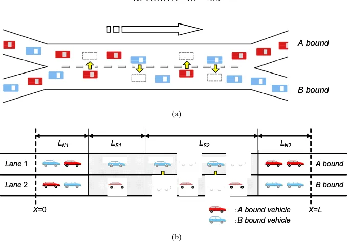
Figure 1(a) shows the schematic illustration of the weav- ing traffic flow through the merging junction on the two- lane highway. A-bound vehicles are indicated by dark (red) color. B-bound vehicles are indicated by light (blue) color. Two kinds of vehicles enter into the merging junc- tion together. The weaving occurs at the merging section. Vehicles move ahead by changing their lane if necessary. Vehicles slow down to change their lane when they enter into the weaving (merging) section. Figure 1(b) shows the schematic illustration of the weaving traffic flow model on the two-lane highway.

We partitioned the two-lane highway with the merging junction into four sections. Section N1 is a normal region with maximal velocity vf,max where vehicles do not

change their lane. Section S1 is a slowdown region with maximal velocity vf,max (





vehi-cles do not change their lane but slow down. Section S2 is a weaving region with maximal velocity s1,max where

vehicles change their lane if necessary. Section N2 is an acceleration region with maximal velocity f,max where

vehicles do not change their lane but speed up. The lengths of Sections N1, S1, S2, and N2 are set as

1 1 2 2

v v

, , ,

N S S N

L L L L respectively. Two kinds of vehicles enter into the two-lane highway with mixing at a fraction. Vehicles slow down when they enter into Section S1. In Section S2, they change their lane with slowing down if necessary. After changing the lane, vehicles go ahead with accelerating.

Here, traffic flow is under the periodic boundary con- dition. In real traffic, vehicular traffic is under the open boundary. The open boundary condition affects the traf- fic behavior. Also, under the open boundary conditions, it is not easy to vary the values of vehicular density. To study the effect of the vehicular density on the traffic flow, one uses the periodic boundary condition.

We assume that vehicles are forced to slow down when they enter into sections of the slowdown and weaving. When vehicles enter into the weaving section S2, vehicles change their lane if the criteria of lane changing are satisfied. The speed is lower, the lane changing is easier. At highway junctions in Japan, the slowdown region is set just before the weaving region because the lane changing is easy. Therefore, we set the slowdown section just before the weaving section. In the weaving section, vehicles slow down and change the lane. Even if there exist no slowdown section, the present simulation result is effective because vehicles slow down in the weaving section.

A bound

B bound A bound

B bound

(a)

X=0 X=L

LN1 LN2

Lane1

Lane2

LS1

：A bound vehicle LS2

A bound

B bound

：B bound vehicle

X=0 X=L

LN1 LN2

Lane1

Lane2

LS1

：A bound vehicle LS2

A bound

B bound

：B bound vehicle

(b)

Figure 1. (a) Schematic illustration of the weaving traffic flow through the merging and bifurcating junction on the two-lane highway. A-bound vehicles are indicated by dark (red) color. B-bound vehicles are indicated by light (blue) color. Two kinds of vehicles enter into the junction with a mixed state. The weaving occurs at the merging section; (b) Schematic illustration of the weaving traffic flow model on the two-lane highway. We partitioned the two-lane highway with the junction into four sections.

enters into the desired lane, the vehicular speed and headway vary with time continuously. In weaving traffic, it is necessary and important that the physical quantities, space, and time are continuous variables. We prefer the differential equation model rather than the CA model. In the traffic model described in terms of the differential equation, the optimal velocity model is simple and is well studied. Therefore, we applied the optimal velocity model to the weaving traffic. Since the original optimal velocity model is an over-simplified model, we extended the original optimal velocity model to take into account the bottleneck effect (slowdown) and the lane changing.

Lane changing is implemented as a sideways move- ment. We assume that the vehicular movement is divided into two parts: one is the forward movement and the oth-er is the sideways movement. We apply the optimal ve- locity model to the forward movement [1,15]. The opti- mal velocity model is described by the following equa- tion of motion of vehicle i :

 

2

d

d d

i

i d _i

x x

a V x

t t



 _  

 

 



, (1)

where V



 

the position of vehicle i at time t,

 



 

 

i i i



x t x_ t x t

  

a

is the headway of vehicle i at time t, and is the sensitivity (the inverse of the delay time) [1].

A driver adjusts the vehicular speed to approach the optimal velocity determined by the observed headway. The sensitivity allows for the time lag a 1 a that

it takes the vehicular speed to reach the optimal velocity when the traffic is varying. Generally, it is necessary that the optimal velocity function has the following properties: it is a monotonically increasing function and it has an upper bound (maximal velocity). The vehicle length is taken to be zero.

Vehicles move with the normal velocity except for the slowdown sections. In the region of normal-speed section, the optimal velocity function of vehicles is given by

 







, ,

tanh tanh

2

f

i i f c f c

v

V x  _  x x  x



roadway except for the slowdown sections and v

, f c

x the position of turning point [1].

In the slowdown Section S1 and weaving Section S2, vehicles move with the forced speed and the vehicular velocity should be lower than the speed limits of slow-down. When vehicles enter into the slowdown and weav- ing sections, they obey the conventional optimal-velocity function with speed limit vs,max:

 







,

tanh tanh

2

s

i i s c

v

V x  _  x x  x_{s c,}



where s,max is the speed limit of slowdown and

weav-ing sections, v

,max ,max

s f

v v , and xs c, the position of

turning point.

driver of A-bound (B-bound) vehicle on the second (first) lane change to the first (second) lane if the security crite-rion is satisfied. The security critecrite-rion is necessary to avoid the collision with the vehicles ahead or behind. The space between vehicles ahead and behind should be sufficiently large not to collide with the vehicles ahead and behind. The space is proportional to the maximal velocity. We propose the following security criterion. When the headway between his vehicle and the front vehicle on the target lane is larger than the prescribed distance and the headway between his vehicle and the back vehicle on the target lane is larger than the pre- scribed distance, it is successful for his vehicle to change the lane. We set the prescribed distance as xs c, vs,max 2.

We adopt the following lane changing rule for the two-lane highway:

, ,max 2

f s c s

x x v

  and  xb x vs c s, ,max 2

for the security criterion, (4) where xf is the headway between vehicle i and the

vehicle ahead on the target lane and xb is the headway

between vehicle i and the vehicle behind on the target lane. Figure 2(a) shows the schematic illustration of lane changing. After changing lane, the vehicle shifts just to the side in Figure 2(a).

If the security criterion (4) is not satisfied, the follow- ing security rule is applied because the vehicle acceler- ates or decelerates for changing lane:

, ,max

f b s c s

x x x v

    for the security condition. (5)

Figure 2(b) shows the schematic illustration of lane changing. After changing lane, the vehicular position on the target lane changes to the following:









2 if ,

2 if .

i i f b f b

i i b f f b

x x x x x x

x x x x x x

       

        (6)

The dynamics is determined by Equations (1)-(6). Then, various dynamic states of traffic appear and traffic jams may occur. We study the dynamic states, traffic jams, and fundamental diagrams in the traffic flows de- scribed by the model in Figure 1(b).

For later convenience, we summarize the dynamic states and spontaneous jams for the conventional optimal velocity model. The conventional optimal velocity model with a single turning point exhibits two phases and a co- existing state of two phases. Below the critical point









In this paper, we restrict ourselves to such case that sensitivity is higher than the critical point, c, be-

cause we do not investigate the spontaneous jam but study the traffic states induced by weaving.

aa

3. Simulation and Result

We perform computer simulation for the traffic model shown in Figure 1(b). We simulate the traffic flow under the periodic boundary condition. The number of vehicles is constant and conserved on the two-lane highway. When a vehicle goes out of the two-lane highway at x = L, it returns to either lane 1 or lane 2 at x = 0 at proba- bility 1/2. At x = 0, returned vehicles on lanes 1 and 2 are classified into two kinds of vehicles randomly. Vehicles on the first lane at x = 0 become A-bound vehicles at probability cA and B-bound vehicles at probability

1cA where cA is the fraction of A-bound vehicles on

lane 1. Vehicles on the second lane at x = 0 become B-bound vehicles at probability cB and A-bound vehi-

cles at probability 1cB where cB is the fraction of

B-bound vehicles on lane 2. The simulation is performed until the traffic flow reaches a steady state. We solve numerically Equation (1) with optimal velocity functions (2) and (3) under lane changing criteria (4)-(6) by using fourth-order Runge-Kutta method where the time interval is  t 1 128. We assume that vehicles try to change their lane every tchange. We set tchange80.

We carry out simulation by varying the vehicular den- sity for road length L = 500, sensitivity , maxi- mal velocities

7.0 a

,max 2.0 f

v  and ,max , and

safety distance , ,

0.8,1.0,1.2

s

v 

4.0

f c s c

x x 

0.7

A B

c c

. First, we study the traf- fic behavior for the symmetric case (cA B). Figure 3(a) shows the plots of traffic currents on lane 1 against density at

c



  and vs,max1.0 where

100

N

L  , LS1100, LS2200, and LN2100. In (a)

i i1

i

x



b

x

 xf

i i1

i

x



b

x

 xf

i i1

i

x



b

x

 xf

i i1

i

x



b

x

 xf

(a) (b)

0.7

A B

c c 

2.

f

v 

, 30 percent vehicles on lanes 1 and 2 try to change their lane. The traffic currents are given for x = L. The density is the mean density over Sections N1, S1, S2, and N2. The open (red) and full (blue) circles indicate, respectively, the traffic currents of A-bound and B-bound vehicles on the first lane obtained by simulation. The open (green) triangles indicate the sum of traffic currents of A-bound and B-bound vehicles on the first lane. The upper solid curve represents the theoretical current curve for ,max without slowdown sections. The lower

solid curve represents the theoretical current curve for all slowdown sections of

0

,max 1.0 s

v  . The theoretical cur- rent is given by





V x

J x

 

 , (7)

where the optimal velocities at the normal and slow speeds are presented by Equations (2) and (3) respect- tively and xint

v

is the initial headway.

If one takes max = 2.0 as maximal velocity 90 km/h

and unit length as 10m, the maximal current is 150 vehi- cles/5 minutes and its density is 20 vehicles/km. These values agree with real traffic data. Thus, one can translate the dimensionless quantities to the typical values.

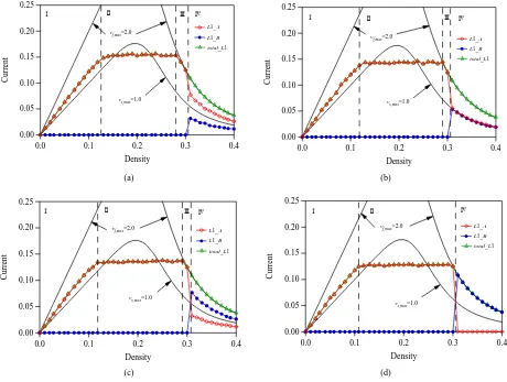
Open (red) circles represent the currents of A-bound vehicles sorting successfully into the first lane. Full (blue) circles represent the currents of B-bound vehicles failed to sorting into the second lane. In this symmetric case, the current of A-bound vehicles on the first lane is con-sistent with that of B-bound vehicles on the second lane. Also, the current of B-bound vehicles on the first lane is consistent with that of A-bound vehicles on the second lane. Traffic states change with increasing density through the dynamical phase transitions. Traffic is classified into four states. The boundaries among the distinct traffic states give the transition points. In region Ⅰ at low den- sity, all vehicles move nearly with the maximal velocity

,max and vehicles sort successfully into the re-

spective lanes. In region Ⅱ, the currents of A-bound and B-bound vehicles on first and second lanes saturate and keep a constant value. A-bound (B-bound) vehicles sort successfully into the first (second) lane. In region Ⅲ, the current of A-bound (B-bound) vehicles on the first (sec- ond) lane decreases with increasing density. A-bound and B-bound vehicles are successful to sort into the re- spective lanes. In region Ⅳ at high density, the currents decrease with increasing density. A-bound and B-bound vehicles mix on both lanes and fail to sort into the re- spective lanes.

2.0

f

v 

We study the effect of fraction cA (cB) on the fun-

damental diagram for the symmetric case. Figures 3(b)-(d)

show the plots of traffic currents on lane 1 against

den-sity at (b) , (c) , and (d)

where , ,

0.5

A B

c c 

,max s

v

0.3



A B

c c

N

L

 

100 0.0

A B

c c  1.0 LS1100,

2 200

S

L  , and LN2100. In (d) , all

vehicles on lanes 1 and 2 try to change their lane. The open (red) and full (blue) circles indicate, respectively, the traffic currents of A-bound and B-bound vehicles on the first lane obtained by simulation. The open (green) triangles indicate the sum of traffic currents of A-bound and B-bound vehicles on the first lane. With decreasing fraction

0.0

A B

c c 

 

A B

c c

c c

, the current of vehicles failed changing lane in region Ⅳ increases. Region Ⅲ does not appear for (d) A B0.0. The transition point between re-

gions Ⅰ and Ⅱ little change with fraction c_A

 

 

than transition point between regions Ⅲand , Ⅳ vehicles fail to sort into the respective lane. The transition point is higher, vehicles are easier to change their lane. This tran- sition point is very important for the traffic control.

We study the traffic patterns and velocity profiles of velocity for distinct traffic states Ⅰ-Ⅳ at cAcB0.7

0.06 shown in Figure 3(a). Diagrams (a)-(d) in Figure 4

show the traffic patterns at (a) density  , (b) 0.15

 , (c) 0.30, and (d) 0.36. The vehicu-lar position is plotted on the two-lane highway at time t = 60000. An A-bound vehicle is indicated by a (red) dot. A B-bound vehicle is indicated by a (blue) bar. Figure 5

shows the plots of velocity against vehicular position on lanes 1 and 2. The velocity profiles on lanes 1 and 2 are plotted by open (red) and full (blue) circles respectively. Diagrams (a)-(d) are the velocity profiles at (a) density

0.06

 , (b) 0.15, (c) 0.30, and (d) 0.36. city profiles (a)-(d) correspond to the traffic patterns (a)-(d) respectively. Figures 4 and 5 are the typical patterns and profiles for distinct traffic states

Ⅰ-Ⅳ in Figure 3(a). Pattern (a) and velocity profile (a) display the free traffic with no jam where all vehicles are successful to sort into respective lanes. Pattern (b) and velocity profile (b) exhibit the jammed state. The jam extends from slowdown Section S1 to normal Section N1. Also, all vehicles are successful to sort into respective lanes. Pattern (c) and velocity profile (c) display the congested state. The jam extends over the whole highway. Irrespective of the congestion, all vehicles are successful to sort into respective lanes. Pattern (d) and velocity pro- file (d) exhibit more congested state than pattern (c). Ve-hicles fail to sort into the respective lanes. A-bound and B-bound vehicles are mixed on lanes 1 and 2 at Section N2.

The velo

0.25

0.20

0.15

0.10

0.05

0.00

Cu

rren

t

0.4 0.3

0.2 0.1

0.0

Density

L1_A

L1_B

total_L1

Ⅰ Ⅱ Ⅲ

v_f,max=2.0

vs,max=1.0

Ⅳ 0.25

0.20

0.15

0.10

0.05

0.00

Current

0.4 0.3

0.2 0.1

0.0

Density

Ⅰ Ⅱ Ⅲ

L1_A

L1_B

total_L1

vs,max=1.0 vf,max=2.0

Ⅳ

(a) (b)

0.25

0.20

0.15

0.10

0.05

0.00

C

urre

nt

0.4 0.3

0.2 0.1

0.0

Density

L1_A

L1_B

total_L1

Ⅰ Ⅱ Ⅲ

vf,max=2.0

vs,max=1.0

Ⅳ

0.25

0.20

0.15

0.10

0.05

0.00

Cu

rre

n

t

0.4 0.3

0.2 0.1

0.0

Density

L1_A

L1_B

total_L1

Ⅰ Ⅱ Ⅳ

vf,max=2.0

vs,max=1.0

(c) (d)

Figure 3. Plots of traffic currents on lane 1 against density at (a) cA = cB = 0.7; (b) cA = cB = 0.5; (c) cA = cB = 0.3; and (d) cA = cB = 0.0, where vs,max = 1.0, LN = 100, LS1 = 100, LS2 = 200, and LN2 = 100. Open (red) circles represent the currents of A-bound vehicles sorting successfully into the first lane. Full (blue) circles represent the currents of B-bound vehicles failed to sorting into the second lane. The upper solid curve represents the theoretical current curve for vf,max = 2.0 without slowdown sections. The lower solid curve represents the theoretical current curve for all slowdown sections of vs,max = 1.0.

2 1

Lane nu

mber

500 400

300 200

100 0

Position

2 1

L

ane

nu

m

b

er

500 400

300 200

100 0

Position (a) (b)

2 1

L

ane num

ber

500 400

300 200

100 0

Position

2 1

La

ne

numbe

r

500 400

300 200

100 0

Position

(c) (d)

2.0

1.5

1.0

0.5

0.0

Ve

lo

city

500 400

300 200

100 0

Position

Lane1

Lane2

N1 S1 S2 N2

2.0

1.5

1.0

0.5

0.0

Velocity

500 400

300 200

100 0

Position

N1 S1 S2 N2

Lane1

Lane2

(a) (b)

2.0

1.5

1.0

0.5

0.0

Veloci

ty

500 400

300 200

100 0

Position

N1 S1 S2 N2

Lane1

Lane2

2.0

1.5

1.0

0.5

0.0

Velo

city

500 400

300 200

100 0

Position

Lane1

Lane2

N1 S1 S2 N2

(c) (d)

Figure 5. Plots of velocity against vehicular position on lanes 1 and 2. The velocity profiles on lanes 1 and 2 are plotted by open (red) and full (blue) circles respectively. Diagrams (a)-(d) are the velocity profiles at (a) density ρ = 0.06; (b) ρ = 0.15; (c)

ρ = 0.30; and (d) ρ = 0.36. The velocity profiles (a)-(d) correspond to the traffic patterns (a)-(d) respectively.

take their desired route at a high density due to no possi- bility of the lane changing.

We study the effect of slowdown speed on the traffic behavior and fundamental diagram. We investigate the dependence of the dynamical transitions on the slow- down speed. Figure 6(a) shows the plots of traffic cur- rents on lane 1 against density at and slow-

down speed where , 1

0.7

A B

c c  100

N

L 

,max 0.8 s

v  LS 100,

2 , and 2 . Figure 6(b) shows the plots

of traffic currents on lane 1 against density at and slowdown speed s,max . The

open (red) and full (blue) circles indicate, respectively, the traffic currents of A-bound and B-bound vehicles on the first lane obtained by simulation. The open (green) triangles indicate the sum of traffic currents of A-bound and B-bound vehicles on the first lane. The upper solid curve represents the theoretical current curve for

,max without slowdown sections. In Figure 6(a),

the lower solid curve represents the theoretical current curve for all slowdown sections of s,max . In Fig- ure 6(b), the lower solid curve represents the theoretical current curve for all slowdown sections of

200

S

L 

A B

c c 

2.0

f

v 

100

N

L 

0.7 1.2

8

,max 1.2

v 

0.

v 

s

v  .

When the slowdown speed decreases, the value of max- imal current (saturated current) becomes lower and the transition point between traffic states Ⅱ and Ⅲ is higher. With decreasing slowdown speed vs,max, the maximal

current decreases. However, the sorting (lane changing) is possible until higher density. If drivers slow down until lower speed, they are successful to sort into respective lanes at higher density.

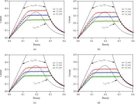
We study the effect of both slowdown speed and frac-tion on the fundamental diagram. Figure 7 shows the plots of total current on lane 1 against density where

100

N

L  , LS1100, LS2200, and 2 . The

total current is given by the sum of currents of A-bound and B-bound vehicles on lane 1. The total current on lane 2 equals that on lane 1 in the symmetric case. Diagrams (a)-(d) in Figure 7 show the plots of total currents on lane 1 against density for slowdown speeds

100

N 

L

,max 1.2,1.0, 0.8 s

v  at (a) fraction cAcB0.7, (b) 0.5

A B

c c  , (c) cAcB0.3, and (d) cAcB0.0.

Open (red) circles, open (blue) triangles, and open (green) squares indicate the total currents for slowdown speeds

,max 1.2,1.0, 0.8 s

0.25

0.20

0.15

0.10

0.05

0.00

Cu

rr

e

n

t

0.4 0.3

0.2 0.1

0.0

Density

Ⅰ Ⅱ Ⅲ

vf,max=2.0

vs,max=0.8

L1_A

L1_B

total_L1

Ⅳ 0.25

0.20

0.15

0.10

0.05

0.00

Cu

rr

e

n

t

0.4 0.3

0.2 0.1

0.0

Density

Ⅰ Ⅱ vf,max=2.0 Ⅳ

vs,max=1.2

L1_A

L1_B

total_L1

(a) (b)

Figure 6. Plots of traffic currents on lane 1 against density at cA = cB = 0.7 and slowdown speed (a) vs,max = 0.8 and (b) vs,max = 1.2 where LN = 100, LS1 = 100, LS2 = 200, and LN2 = 100. The open (red) and full (blue) circles indicate, respectively, the traffic currents of A-bound and B-bound vehicles on the first lane obtained by simulation. The open (green) triangles indicate the sum of traffic currents of A-bound and B-bound vehicles on the first lane.

0.5

0.4

0.3

0.2

0.1

0.0

Cu

rr

en

t

0.4 0.3

0.2 0.1

0.0

Density

0.8_total 1.0_total 1.2_total vf,max=2.0

vs,max=1.0

0.5

0.4

0.3

0.2

0.1

0.0

Cu

rren

t

0.4 0.3

0.2 0.1

0.0

Density

0.8_total 1.0_total 1.2_total vf,max=2.0

vs,max=1.0

(a) (b)

0.5

0.4

0.3

0.2

0.1

0.0

Cu

rr

ent

0.4 0.3

0.2 0.1

0.0

Density

0.8_total 1.0_total 1.2_total vf,max=2.0

vs,max=1.0

0.5

0.4

0.3

0.2

0.1

0.0

Cu

rr

en

t

0.4 0.3

0.2 0.1

0.0

Density

0.8_total 1.0_total 1.2_total vf,max=2.0

vs,max=1.0

(c) (d)

Figure 7. Plots of total current on lane 1 against density where LN = 100, LS1 = 100, LS2 = 200, and LN2 = 100. Diagrams (a)-(d) show the plots of total currents on lane 1 against density for slowdown speeds vs,max = 1.2, 1.0, 0.8 at (a) fraction cA = cB = 0.7; (b) cA = cB = 0.5; (c) cA = cB = 0.3; and (d) cA = cB = 0.0. Open (red) circles, open (blue) triangles, and open (green) squares indi-

ate the total currents for slowdown speeds vs,max = 1.2, 1.0, 0.8 respectively. c

represents the theoretical current for ,max . When

the fraction decreases, the number of vehicles trying the lane changing increases. With decreasing fraction , the maximal current (saturated current) de-creases. This is due to the following reason. When the vehicles changing the lane increases, the headway be-comes shorter at lane-changing Section S2. The speed reduces by shorter headway. The reduced speed results in the lower maximal current.

1.0

s

v 

 

A B

c c

We study the effect of length S2 at weaving Section

S2 on the fundamental diagram. Figure 8 shows the fundamental diagrams for (a) , (b)

l

2

S 200

l lS2100,

and (c) where , ,

, 1 , and N2 . Open (red) and

full (blue) circles indicate the currents of A-bound and B-bound vehicles on lane 1 respectively. Open (green) triangles represent the total current (sum) of A-bound and B-bound vehicles on lane 1. Vehicles try to change their lane every c time. In cases (a) and (b)

that weaving length is larger than

2 50

S

l  10

S

L 

80

t v 

,max1.0

100



s

v L

80



0.5

A B

c c  100

N

L 

 

0

h

t



l 1

ange S

 2, the fundamental diagram does

not depend on change

change s,max

t

 because the weaving length is sufficiently large for vehicles to change their lane. In case (c), B-bound (A-bound) vehicles on lane 1 (lane 2) failed to change their lane within the weaving section because there is not a sufficient length for vehicles to change their lane. Thus, it is necessary and important that the length of weaving section is sufficiently larger than

change s,max

t v

 

p

.

We consider the asymmetric case that the inflow on lane 1 is definitely different from that on lane 2. In the asymmetric case, when a vehicle goes out of the two-lane highway at x = L, it returns to lane 1 at x = 0 at probabil-ity r and to lane 2 at x = 0 at probability 1pr. The

symmetric case is pr0.5. Furthermore, returned cles on lane 1 (lane 2) become A-bound (B-bound) vehi-cles at probability A

 



p

c c and B-bound vehicles (A- bound) at probability . Figure 9 shows the fundamental diagrams for where



1 c_A 1c_B 0.3

r



0.7

A B

c c  ,

,max 1.0 s

v  , L_N 100, 1 , S2 , a n d

2

100

S 

L L 200

100 N

L  . Diagram (a) shows the plots of currents on lane 1 against density. Open (red) and full (blue) circles

0.25

0.20

0.15

0.10

0.05

0.00

Cu

rr

en

t

0.4 0.3

0.2 0.1

0.0

Density

Ⅰ Ⅱ Ⅲ

L1_A

L1_B

total_L1

vs,max=1.0 vf,max=2.0

Ⅳ

0.25

0.20

0.15

0.10

0.05

0.00

Cu

rren

t

0.4 0.3

0.2 0.1

0.0

Density

Ⅰ Ⅱ Ⅲ

L1_A

L1_B

total_L1 vf,max=2.0

Ⅳ

v_s,max=1.0

(a) (b)

0.25

0.20

0.15

0.10

0.05

0.00

Curre

nt

0.4 0.3

0.2 0.1

0.0

Density

Ⅰ Ⅱ Ⅲ

L1_A

L1_B

total_L1 vf,max=2.0

Ⅳ

vs,max=1.0

(c)

0.25

0.20

0.15

0.10

0.05

0.00

Cu

rr

en

t

0.4 0.3

0.2 0.1

0.0

Density

L1_A

L1_B

total_L1

Ⅰ Ⅱ Ⅲ

vf,max=2.0

vs,max=1.0

Ⅳ

0.25

0.20

0.15

0.10

0.05

0.00

Curr

ent

0.4 0.3

0.2 0.1

0.0

Density

L2_A L2_B

total_L2

Ⅰ Ⅱ Ⅲ

vf,max=2.0

vs,max=1.0

Ⅳ

(a) (b)

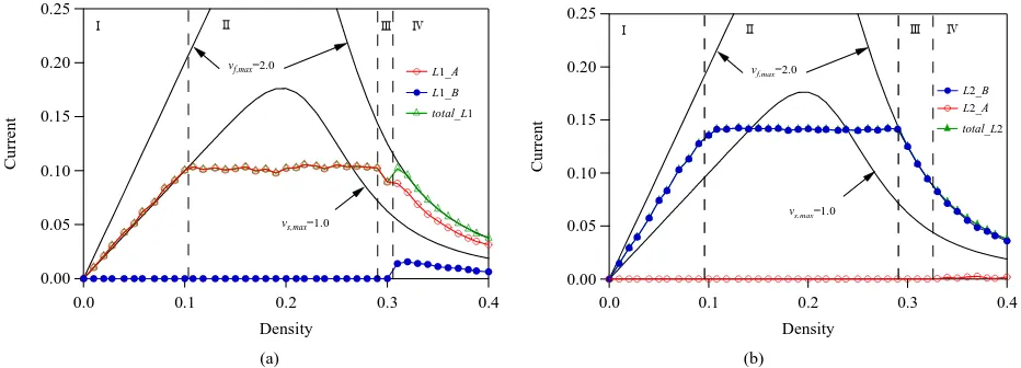
Figure 9. Fundamental diagrams for pr = 0.3 where cA = cB = 0.7, vs,max = 1.0, LN = 100, LS1 = 100, LS2 = 200, and LN2 = 100. Diagram (a) shows the plots of currents on lane 1 against density. Open (red) and full (blue) circles indicate the currents of A-bound and B-bound vehicles on lane 1 respectively. Diagram (b) represents the plots of currents on lane 2 against density. Full (blue) and open (red) circles indicate the currents of B-bound and A-bound vehicles on lane 2 respectively.

indicate the currents of A-bound and B-bound vehicles on lane 1 respectively. Open (green) triangles represent the sum of currents of A-bound and B-bound vehicles on lane 1. Diagram (b) represents the plots of currents on lane 2 against density. Full (blue) and open (red) circles indicate the currents of B-bound and A-bound vehicles on lane 2 respectively. B-bound vehicles on lane 1 failed to change lane 2 when the density is higher than the tran-sition point between traffic states III and IV. The transi-tion point between traffic states III and IV on lane 1 is lower than that on lane 2. B-bound vehicles on lane 1 are hard to change the lane because the second lane is more congested than the first lane. The saturated current on lane 2 is higher than that on lane 1 because B-bound ve-hicles are more than A-bound veve-hicles.

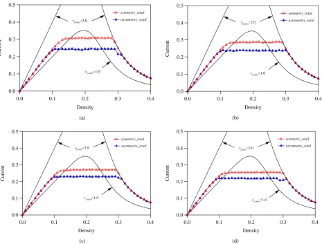
We compare the fundamental diagram of the asym-metric case with that of the symmetric case

. Figure 10 shows the fundamental diagram

where , , 1 , 2

0.3 r

p 

x1.0 L

0.5 r

p 

s

v,ma N 100 LS 100 LS 200,

and N2 . Diagrams (a)-(d) represent the plots of

total current on lane 1 against density for (a) 100

L 

0.7

A B

c c  , (b) _A _B0.5, (c) , and (d)

0.0

c c

c c 

0.3

A B

A B . Open (red) and full (blue) triangles indi-

cate the total current for the symmetric and asymmetric cases respectively. The current for the symmetric case is higher than that for the asymmetric case because the lane 2 is more congested than the lane 1 for the asymmetric case.

c c 

Thus, the traffic states and fundamental diagram for the weaving traffic vary with the density, the slowdown speed, and the fraction of vehicles changing the direction. A traffic state changes to different states through some dynamical phase transitions. The traffic flow in the weaving traffic at the junction shows the very complex behavior. In order to sort successfully into the respective

lanes, it is necessary and important for the vehicular den-sity to be lower than the relevant transition point.

We note the traffic flow under the open-boundary con-dition. Real-world traffic is under open boundary tions, while our model is under periodic boundary condi-tions. The traffic flow with open boundary conditions is mainly determined by inflow and outflow densities. If the outflow density is low, the traffic behavior is governed by the inflow density. In the traffic model with periodic boundary condition, the traffic flow is governed by the mean density where the mean density is defined by [total number of vehicles]/[road length]. In traffic states at a steady state, the traffic phases for periodic boundary conditions are related to those for open boundary condi-tions via the mean density. When the outflow density is low, the inflow density is proportional to the mean den-sity. The fundamental diagram of flow vs. inflow density under open boundary conditions is similar to that of flow vs. mean density under periodic boundary conditions. If the inflow density is translated to the mean density, the steady-state phases under open boundary conditions are relevant to those under periodic boundary conditions for the same value of mean density.

We perform the simulation for the open boundary con-dition. We derive the fundamental diagram for the open boundary condition. We compare the open-boundary traffic with the closed-boundary traffic. Figure 11(a)

0.5

0.4

0.3

0.2

0.1

0.0

C

urr

ent

0.4 0.3

0.2 0.1

0.0

Density

vf,max=2.0

vs,max=1.0

symmetry_total

asymmetry_total

0.5

0.4

0.3

0.2

0.1

0.0

Cu

rren

t

0.4 0.3

0.2 0.1

0.0

Density

vf,max=2.0

vs,max=1.0

symmetry_total

asymmetry_total

(a) (b)

0.5

0.4

0.3

0.2

0.1

0.0

Cu

rr

en

t

0.4 0.3

0.2 0.1

0.0

Density

vf,max=2.0

vs,max=1.0

symmetry_total

asymmetry_total

0.5

0.4

0.3

0.2

0.1

0.0

Cu

rr

en

t

0.4 0.3

0.2 0.1

0.0

Density

vf,max=2.0

vs,max=1.0

symmetry_total

asymmetry_total

(c) (d)

Figure 10. Fundamental diagram where vs,max = 1.0, LN = 100, LS1 = 100, LS2 = 200, and LN2 = 100. Diagrams (a)-(d) represent the plots of total current on lane 1 against density for (a) cA = cB = 0.7; (b) cA = cB = 0.5; (c) cA = cB = 0.3; and (d) cA = cB = 0.0. Open (red) and full (blue) triangles indicate the total current for the symmetric and asymmetric cases respectively.

boundary condition, Figure 11(c) is obtained by using

Figure 11(b). Open circles indicate the simulation result of open boundary and the solid curve represents that of periodic boundary. The open-boundary result agrees roughly with the periodic-boundary result. However, the high-density phase does not appear. Thus, the peri-odic-boundary traffic flow will be applied to the real- word traffic.

If the inflow density is higher than the outflow density under open boundary conditions, the high density state does not occur but the low density state occurs (see Fig- ure 11). Under periodic boundary conditions, two pos- sible states depend on the mean density.

We applied the simplified rules to the lane changing. Generally, the vehicular motion of lane changing is very complex. In order to make the present model better, it will be necessary to improve the lane changing rules. Also, we mimicked the junction by two lanes. However, the junction in real traffic is composed of four lanes higher than two lanes. It will be necessary to extend the

present model to the junction on four lanes.

4. Summary

We have investigated the traffic states and dynamical phase transitions in the merging and bifurcating traffic flow (weaving traffic) at the junction on a two-lane highway. We have presented the dynamical traffic model mimicking the weaving traffic at the junction. We have derived the fundamental diagrams (current-density dia-grams) for the traffic flow on the weaving traffic. We have shown that there are four distinct traffic states and the traffic flow changes to the distinct states through three dynamical transitions. We have found the condition such that vehicles changing the direction are successful to sort themselves into their respective lanes. We have clarified that the traffic flow depends highly on the ve-hicular density, the slowdown speed, and the fraction of vehicles changing the direction.

0.4

0.3

0.2

0.1

0.0

Current

0.4 0.3

0.2 0.1

0.0

Inflow density

Theoretical line Weaving current Open boundary

0.4

0.3

0.2

0.1

0.0

Mean d

ens

ity

0.4 0.3

0.2 0.1

0.0

Inflow density Open boundary

(a) (b)

0.4

0.3

0.2

0.1

0.0

Cu

rren

t

0.4 0.3

0.2 0.1

0.0

Mean density

Weaving current Periodic boundary

Open boundary

(c)

Figure 11. (a) Plot of current against inflow density for the open-boundary traffic where outflow density is zero. Open circles indicate the simulation result. The solid line represents the theoretical current curve; (b) Plot of mean density against inflow density; (c) Plot of current against mean density for the open boundary condition.

merging and bifurcating vehicles and to clarify the de- pendence of successful weaving traffic on the slowdown speed. This work will be useful to operate efficiently the junction on the highway.

REFERENCES

[1] T. Nagatani, “The Physics of Traffic Jams,” Reports on Progress Physics, Vol. 65, No. 9, 2002, pp. 1331-1386.

doi:10.1088/0034-4885/65/9/203

[2] D. Helbing, “Traffic and Related Self-Driven Many-Par- ticle Systems,” Reviews of Modern Physics, Vol. 73, No. 4, 2001, pp. 1067-1141.

doi:10.1103/RevModPhys.73.1067

[3] D. Chowdhury, L. Santen and A. Schadscheider, “Statis- tical Physics of Vehicular Traffic and Some Related Sys- tems,” Physics Report, Vol. 329, No. 4, 2000, pp. 199- 329. doi:10.1016/S0370-1573(99)00117-9

[4] K. Nagel and M. Schreckenberg, “A Cellular Automaton Model for Freeway Traffic,” Journal of Physics I France, Vol. 2, No. 12, 1992, pp. 2221-2229.

doi:10.1051/jp1:1992277

[5] M. Treiber, A. Hennecke and D. Helbing, “Congested Traffic States in Empirical Observations and Microscopic Simulations,” Physical Review E, Vol. 62, No. 2, 2000, pp. 1805-1824. doi:10.1103/PhysRevE.62.1805

[6] K. Nishinari, D. Chowdhury and A. Schadschneider, “Cluster Formation and Anomalous Fundamental Dia- gram in an Ant-Trail Model,” Physical Review E, Vol. 67, No. 3, 2002, pp. 1-11. doi:10.1103/PhysRevE.67.036120

[7] K. Yamamoto, S. Kubo and K. Nishinari, “Simulation for Pedestrian Dynamics by Real-Coded Cellular Automata (RCA),” Physica A, Vol. 379, No. 2, 2007, pp. 654-660.

doi:10.1016/j.physa.2007.02.040

[8] T. Nagatani, “Chaotic and Periodic Motions of a Cyclic Bus Induced by Speedup,” Physical Review E, Vol. 66, No. 4, 2002, pp. 1-7. doi:10.1103/PhysRevE.66.046103

[9] E. Brockfeld, R. Barlovic, A. Schadschneider and M. Schreckenberg, “Optimizing Traffic Lights in a Cellular Automaton Model for City Traffic,” Physical Review E, Vol. 64, No. 5, 2001, pp. 1-12.

doi:10.1103/PhysRevE.64.056132

doi:10.1016/S0378-4371(02)01376-6

[11] S. Lammer and D. Helbing, “Self-Control of Traffic Lights and Vehicle Flows in Urban Road Networks,” Journal of Statistical Mechanics: Theory and Experiment, Vol. 2008, No. 4, 2008, pp. 1-36.

doi:10.1088/1742-5468/2008/04/P04019

[12] H. X. Ge, S. Q. Dai, L. Y. Dong and Y. Xue, “Stabiliza-tion Effect of Traffic Flow in an Extended Car-Following Model Based on an Intelligent Transportation System Application,” Physical Review E, Vol. 70, No. 6, 2004, pp. 1-6. doi:10.1103/PhysRevE.70.066134

[13] R. Nagai, T. Nagatani and A. Yamada, “Phase Diagram in Multi-Phase Traffic Model,” Physica A, Vol. 355, No. 2, 2005, pp. 530-550. doi:10.1016/j.physa.2005.04.004

[14] R. Nagai, H. Hanaura, K. Tanaka and T. Nagatani, “Dis- continuity at Edge of Traffic Jam Induced by Slowdown,” Physica A, Vol. 364, No. 2, 2006, pp. 464-472.

doi:10.1016/j.physa.2005.09.055

[15] M. Bando, K. Hasebe, A. Nakayama and Y. Sugiyama, “Dynamical Model of Traffic Congestion and Numerical Simulation,” Physical Review E, Vol. 51, No. 2, 1995, pp. 1035-1042. doi:10.1103/PhysRevE.51.1035

[16] C.-F. Dong, X. Ma and B.-H. Wang, “Weighted Conges-tion Coefficient Feedback in Intelligent TransportaConges-tion Systems,” Physics Letters A, Vol. 374, No. 11, 2010, pp. 1326-1331. doi:10.1016/j.physleta.2010.01.011

[17] R. Jiang, Q. Wu and Z. Zhu, “Full Velocity Difference Model for a Car-Following Theory,” Physical Review E, Vol. 64, No. 1, 2002, pp. 1-4.

doi:10.1103/PhysRevE.64.017101

[18] B. A. Toledo, V. Munoz, J. Rogan and C. Tenreino, “Modeling Traffic through a Sequence of Traffic Light,” Physical Review E, Vol. 70, No. 1, 2004, pp. 1-6.

[19] T. Nagatani, “Clustering and Maximal Flow in Vehicular Traffic through a Sequence of Traffic Lights,” Physica A, Vol. 377, No. 2, 2007, pp. 651-660.

doi:10.1016/j.physa.2006.11.028

[20] C. Chen, J. Chen and X. Guo, “Influences of Overtaking on Two-Lane Traffic with Signals,” Physica A, Vol. 389, No. 1, 2010, pp. 141-148.

doi:10.1016/j.physa.2009.09.007

[21] G. H. Peng, X. H. Cai, B. F. Cao and C. Q. Liu, “Non-

Lane-Based Lattice Hydrodynamic Model of Traffic Flow Considering the Lateral Effects of the Lane Width,” Phy- sics Letters A, Vol. 375, No. 30-31, 2011, pp. 2823-2827.

doi:10.1016/j.physleta.2011.06.021

[22] G. H. Peng, X. H. Cai, C. Q. Liu, B. F. Cao and M. X. Tuo, “Optimal Velocity Difference Model for a Car-Fol- lowing Theory,” Physics Letters A, Vol. 375, No. 45, 2011, pp. 3973-3977. doi:10.1016/j.physleta.2011.09.037

[23] W.-X. Zhu and E.-X. Chi, “Analysis of Generalized Op- timal Current Lattice Model for Traffic Flow,” Interna- tional Journal of Modern Physics C, Vol. 19, No. 5, 2008, pp. 727-739. doi:10.1142/S0129183108012467

[24] Y. Sugiyama, M. Fukui, M. Kikuchi, K. Hasebe, A. Na- kayama, K. Nishinari, S. Tadaki and S. Yukawa, “Traffic Jams without Bottlenecks-Experimental Evidence for the Physical Mechanism of the Formation of a Jam,” New Journal of Physics, Vol. 10, No. 3, 2008, pp. 1-7.

doi:10.1088/1367-2630/10/3/033001

[25] T. Nagatani, “Instability of a Traffic Jam Induced by Slow- ing down,” Journal of Physical Society of Japan, Vol. 66, No. 7, 1997, pp. 1928-1931.

doi:10.1143/JPSJ.66.1928

[26] H. Hanaura, T. Nagatani and K. Tanaka, “Jam Formation in Traffic Flow on a Highway with Some Slowdown,” Physica A, Vol. 374, No. 1, 2007, pp. 419-430.

doi:10.1016/j.physa.2006.07.032

[27] K. Komada, S. Masukura and T. Nagatani, “Traffic Flow on a Toll Highway with Electronic and Traditional Toll- gates,” Physica A, Vol. 388, No. 24, 2009, pp. 4979-4990.

doi:10.1016/j.physa.2009.08.019

[28] R. Nishi, H. Miki, A. Tomoeda and K. Nishinari, “Achieve- ment of Alternative Configurations of Vehicles on Multi- ple Lanes,” Physical Review E, Vol. 79, No. 6, 2009, pp. 1-8. doi:10.1103/PhysRevE.79.066119

[29] H. Kita, “A Merging-Giveway Interaction Model of Cars in a Merging Section: A Game Theoretic Analysis,” Trans- portation Research A, Vol. 33, No. 3, 1999, pp. 305-312.

doi:10.1016/S0965-8564(98)00039-1

[30] P. Hidas, “Modeling Vehicle Interactions in Microscopic Simulation of Merging and Weaving,” Transportation Re- search C, Vol. 13, No. 1, 2005, pp. 37-62.