ISSN Print: 2327-4352
DOI: 10.4236/jamp.2018.66102 Jun. 14, 2018 1215 Journal of Applied Mathematics and Physics
Revenue Optimization of Pipelines
Construction and Operation Management
Based on Quantum Genetic Algorithm and
Simulated Annealing Algorithm
Kang Tan
Department of Civil engineering, Dalian University of Technology, Dalian, China
Abstract
For the optimization of pipelines, most researchers are mainly concerned with designing the most reasonable section to meet the requirements of strength and stiffness, and at the same time reduce the cost as much as possible. It is undeniable that they do achieve this goal by using the lowest cost in design phase to achieve maximum benefits. However, for pipelines, the cost and in-comes of operation management are far greater than those in design phase. Therefore, the novelty of this paper is to propose an optimization model that considers the costs and incomes of the construction and operation phases, and combines them into one model. By comparing three optimization algorithms (genetic algorithm, quantum genetic algorithm and simulated annealing rithm), the same optimization problem is solved. Then the most suitable algo-rithm is selected and the optimal solution is obtained, which provides refer-ence for construction and operation management during the whole life cycle of pipelines.
Keywords
Quantum Genetic Algorithm, Simulated Annealing Algorithm, Pipelines Construction Management, Operation Optimization
1. Introduction
The optimization of infrastructure has been studied by many researchers, focus-ing mainly on the optimization durfocus-ing the design phase, but less on the optimi-zation of pipelines operation and maintenance. Chirehdasta proposed a practical How to cite this paper: Tan, K. (2018)
Revenue Optimization of Pipelines Con-struction and Operation Management Based on Quantum Genetic Algorithm and Simulated Annealing Algorithm. Journal of Applied Mathematics and Physics, 6, 1215-1229.
https://doi.org/10.4236/jamp.2018.66102
Received: May 9, 2018 Accepted: June 11, 2018 Published: June 14, 2018
Copyright © 2018 by author and Scientific Research Publishing Inc. This work is licensed under the Creative Commons Attribution International License (CC BY 4.0).
DOI: 10.4236/jamp.2018.66102 1216 Journal of Applied Mathematics and Physics approach for solving topology optimization problems of planar cross-sections. A problem formulation involving the use of continuous design variables is pre-sented, and a standard nonlinear programming algorithm is used to solve the optimization problem [1]. Liu presented a section topology optimization tech-nique based on an anisotropic beam theory considering warping of sections and coupling among deformations. In formulating the topology optimization prob-lem, the minimum averaged compliance of the beam is taken as objective, and the material density of every element is used as design variable. The scheme is to determine the rigidity matrix of the cross sections and sensitivity analysis [2]. Ren proposed a new topology optimization design method for aircraft composite beam under various loads. To obtain better beam cross section, a multi-material optimization model including anisotropic and isotropic materials is employed. Topology design of composite beam cross section with weight constraint is pre-sented for square and airfoil cross section under various loads. The results show that the proposed method is suitable for the optimization design of composite beam, and innovative structures could be given [3]. Jose presents a novel framework for simultaneous optimization of topology and laminate properties in structural design of laminated composite beam cross sections. The optimiza-tion framework is based on a multi-material topology optimizaoptimiza-tion model in which the design variables represent the amount of the given materials in the cross section. The numerical results suggest that the proposed framework is suitable for simultaneous optimization of cross section topology and identifica-tion of optimal laminate properties in structural design of laminated composite beams [4].
DOI: 10.4236/jamp.2018.66102 1217 Journal of Applied Mathematics and Physics presented a novel formulation aiming to achieve optimal design of reinforced concrete (RC) structures. The design procedures for RC structures that are typi-cally adapted in practice begin by assuming initial stiffness for the structural skeleton elements [8].
Cardoso performs optimal design of cross-section properties of thin-walled laminated composite beams. Design optimization is performed by nonlinear programming techniques. Laminate thickness and lamina orientations are con-sidered as design variables [9]. Cantilever implemented Genetic Algorithm for solving the design optimization problem of Cantilever beam and Torsion rod. Cantilever beam and Torsion rod are used as structural elements in many Me-chanical Engineering applications. The objective here is to design a cantilever beam and a Torsion rod for minimum weight in order to withstand the given working condition [10]. Liu described a second-order shape and cross-section optimization method of plane truss subjected to earthquake excitation. The in-equality time-dependent constraint problem was converted into a sequence of appropriately formed unconstrained problems using the integral interior penalty function method. The results show that the new optimization method is an effi-cient and effective approach for minimum weight design of truss structures [11]. To examine optimal topology of those structural bending members which com-monly possess constant cross section along the axis the topology optimization with extrusion constraint is more appropriate. The extrusion constraint method suggests a fresh approach to investigate optimal topologies of beam cross section under the influence of realistic loading condition across the section at the begin-ning of design cycle. Presented study is focused upon the influence of various configuration and location of the load and boundary [12]. Zhang developed a new method of discrete optimization for cross-section selection of truss struc-tures. The proposed method is applied to several benchmark design examples, generating results with similar or improved accuracy compared to those from heuristic methods, showing significantly improved computational efficiency. The method is shown to be accurate and efficient, which would prove especially beneficial to large-scale problems [13].
DOI: 10.4236/jamp.2018.66102 1218 Journal of Applied Mathematics and Physics for construction and operation management during the whole life cycle of pipe-lines.
2. Methodology
The optimization of the construction and operation management for pipelines is to increase revenue and reduce expenditure so as to achieve the goals of profit maximization during life cycle period. Firstly, we should optimize the design of pipelines. The optimal design of pipelines is generally to optimize the thickness of pipeline and the ratio of reinforcement of pipelines in the conditions of the internal pressure and ground load to determine the most economical and best performance cross sections. Secondly, we should consider the incomes and costs during operation phase. The internal space of pipelines can be leased to pipeline companies for revenue. At the same time, expenses for operation and mainten-ance will also be expended for the maintenmainten-ance of pipelines. Finally, taking into account three factors (construction cost, lease income and operating cost), a simplified optimization model is established and the corresponding constraints are determined to obtain an optimal solution, thereby achieving the goal of prof-it maximization of pipelines.
In the design and construction phase of pipelines, two main factors are consi-dered: one is the thickness, and the other is the ratio of reinforcement. For rein-forced concrete pipelines, the two materials, steel and concrete, differ greatly in terms of prices. If the weight of pipe is the lightest, the designed cross-section will obviously have a small cross-section with high ratio of reinforcement. This design will lead to an increase in construction costs. Therefore, the construction cost can be used as an objective function. In the optimization design of pipelines, in order to simplify the objective function, only the cost of concrete and steel bar is counted. As for other factors such as machine and labor cost are not consi-dered in the objective function.
DOI: 10.4236/jamp.2018.66102 1219 Journal of Applied Mathematics and Physics In summary, for a unit length of reinforced concrete pipe, the objective func-tion and constraint condifunc-tions are
(
)
2 2(
)
(
)
π 2π
c s s
b o
Z C R X R C R a XY R X a XY
C X C X Y
γ
= − + − − + + + −
+ − (1)
min max
T ≤X T≤ (2)
min Y max
ρ ≤ ≤ρ (3) X is the thickness of pipe, Y is the reinforcement ratio of pipe, Cc is the unit price of concrete, Cs is the unit price of steel bar,γs is the density of reinforce-ment concrete, a is the thickness of concrete protection layer, R is the inner ra-dius of pipe, and Cb is the operating incomes factor, Co is the operating expend-itures factor.
For a project case, it can be calculated by specific data.
(
2)
(
)
500π 2 39000π 1.035 0.965
15000 20
Z X X XY X XY
X X Y
= − + − + +
+ − (4)
0.2≤X ≤0.3 (5)
0.004≤ ≤Y 0.025 (6)
3. Genetic Algorithm
3.1. The Principle of Genetic Algorithm
In computer science and operations research, a genetic algorithm (GA) is a me-thod inspired by the process of natural selection that belongs to the larger class of evolutionary algorithms (EA). Genetic algorithms are commonly used to gen-erate high-quality solutions to optimization and search problems by relying on bio-inspired operators such as mutation, crossover and selection [14] [15]. In a genetic algorithm, a population of candidate solutions (called individuals, crea-tures, or phenotypes) to an optimization problem is evolved to better solutions. Each candidate solution has a set of properties (its chromosomes or genotype) which can be mutated and altered. Traditionally, solutions are represented in binary as strings, but other encodings are also possible. An implementation of a genetic algorithm begins with a population of typically random chromosomes. Then evaluates these structures and allocates reproductive opportunities in a way that those chromosomes which represent a better solution to the target problem are given more chances to reproduce than those chromosomes which are poorer solutions. The “goodness” of a solution is typically defined with re-spect to the current population [16] [17].
DOI: 10.4236/jamp.2018.66102 1220 Journal of Applied Mathematics and Physics (recombined and possibly randomly mutated) to form a new generation. The new generation of candidate solutions is then used in the next iteration of the algorithm. Commonly, the algorithm terminates when either a maximum num-ber of generations has been produced, or a satisfactory fitness level has been reached.
3.2. The Process of Genetic Algorithm
The first step of genetic algorithm is population initialization. Since the genetic algorithm cannot directly deal with the parameters of problem, the feasible solu-tion to the problem to be solved must be represented as a chromosome or an in-dividual in the genetic space through coding. Common coding methods are grey coding, real coding, and structural coding. The real number coding does not have to be converted numerically, and the genetic algorithm operation can be performed directly on the expression of the solution. This article uses real cod-ing to define each chromosome as a real variable. Secondly, the fitness function is a criterion to distinguish individual good from bad in a group, and is the only basis for natural selection. Generally, it is obtained by transforming an objective function. This article is to find the maximum value of the function as the indi-vidual fitness value. The larger the value of indiindi-vidual function is, the better the fitness is. Thirdly, the selection operation is to select a good individual from the old group with a certain probability to form a new group to multiply next gener-ation of individuals. The probability that the individual is selected is related to the fitness value. The higher the individual fitness is, the greater the probability of being selected is. There are various methods for selecting the genetic algo-rithm, such as roulette method and competition game method. In this paper, the roulette method is adopted. Fourthly, cross operation refers to randomly select-ing two individuals from population and transferrselect-ing excellent genetic characte-ristics to substrings through the exchange combination of two chromosomes to generate new excellent individuals. Since individuals use real numbers, the cros-sover method uses real number croscros-sover method. Finally, the last step of genet-ic algorithm is mutation operation. The purpose of the mutation operation is to maintain the diversity of the population. The mutation operation randomly se-lects one individual from the population and sese-lects individual to mutate to produce a better individual.
3.3. The Results of Genetic Algorithm
When using genetic algorithms, the four parameters are mainly considered to influence the optimization result. The four parameters are generations, popula-tion, cross possibility and mutation possibility. In order to study the influence of a certain factor on the optimization performance, the interference of other va-riables should be excluded.
DOI: 10.4236/jamp.2018.66102 1221 Journal of Applied Mathematics and Physics
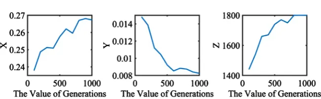
Figure 1. The effects of generations on genetic algorithm.
continue to increase. Although the value will fluctuate in this process, but the general trend is that the value of generations is positively related to X. From the second graph of Figure 1, the value of Y decreases as the value of generations increases. The first half of the curve falls faster, and the latter half declines slow-ly, gradually tends to a fixed value. From the third graph of Figure 1, we can see that the value of Z increases with the value of generations, indicating that in or-der to get optimal solution, you can increase the value of generations. In this way, the entire profit can be maximized.
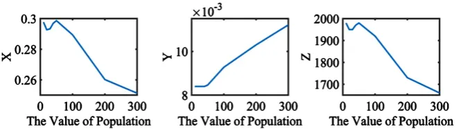
From the first graph of Figure 2, we can see that with the increase of the pop-ulation, the value of X keeps falling, and the downward trend is obvious, but there is a small fluctuation in the beginning part. From the second graph of Fig-ure 2, it can be seen that as the value of population increases, the value of Y
keeps stable at the beginning and gradually increases. The third graph of Figure 2 shows that the shape of the curve is similar to the first graph. Similarly, there is a small fluctuation in the beginning. At this time, the value of Z does not de-crease significantly, and then the value of Z declines fast, indicating that with the increase of the value of population, the value of Z will decrease. Because this ar-ticle seeks the maximum benefit, it means that it will constantly deviate from the optimal solution. Therefore, in order to obtain an optimal solution and obtain maximum benefits during pipeline construction and operation, the value of population should be appropriately reduced.
As can be seen from the first graph of Figure 3, as the cross possibility in-creases, the value of X will continue to increase, but there will be some fluctua-tions in some posifluctua-tions. As can be seen from the second graph of Figure 3, with the increase of cross possibility, the value of Y will continue to decrease. Al-though there will be some minor fluctuations, the overall downward trend of the curve at that time is still obvious. As can be seen from the third graph of Figure 3, as the cross possibility increases, the value of Z continues to increase, indicat-ing that increasindicat-ing the value of cross possibility can make the current value close to the optimal solution. However, compared to other factors, adjusting the value of cross possibility dose not bring significant effect to increase the value of Z and overall profit.
DOI: 10.4236/jamp.2018.66102 1222 Journal of Applied Mathematics and Physics
[image:8.595.218.533.323.408.2]Figure 2.The effects of population on genetic algorithm.
Figure 3.The effects of cross possibility on genetic algorithm.
Figure 4.The effects of mutation possibility on genetic algorithm.
the value of X still shows a decreasing trend. From the second graph of Figure 4, it can be seen that with the increase of mutation possibility, the value of Y de-creases sharply, but in the subsequent part, Y gradually tend to be flattened. Combined with the first and second graphs, it can be seen that the increase of mutation possibility causes X and Y to decrease at the same time. From the third graph of Figure 4, it can be seen that with the increase of mutation possibility, Z
keeps dropping, but there will be some fluctuations in multiple points, and the solution obtained will gradually deviate from the optimal solution. In order to get the best solution and get the maximum benefit, we should try to control the value of mutation possibility, making it within a reasonable range.
4. Quantum Genetic Algorithm
4.1. The Principle of Quantum Genetic Algorithm
DOI: 10.4236/jamp.2018.66102 1223 Journal of Applied Mathematics and Physics quantum algorithm are a combination between GA and quantum computing. They are mainly based on qubits and states superposition of quantum mechan-ics. Unlike the classical representation of chromosomes (binary string for in-stance), here they are represented by vectors of qubits (quantum register). Thus, a chromosome can represent the superposition of all possible states [19]. Genes are modelled upon the concept of qubits, which brings an additional element of randomness and a “new dimension” into the algorithm. The qubit is a basic unit of quantum information. It is a normalised vector in two dimensional vector space spanned by the base vectors 0 and 1. With some simplifications (imaginary part omitted) a state of qubit can be illustrated by a normalized vector on the two-dimensional space. In the beginning of the algorithm the genes of all indi-viduals in the quantum population are initialized with linear superposition. The evaluation of individual’s fitness in the algorithm is performed by observation. In this step the search space is sampled with respect to the probability distribu-tions encoded by quantum individuals. The genetic operators applied in the al-gorithm are based on quantum rotation gates, which rotate state vectors in the quantum gene state space [20].
4.2. The Process of Quantum Genetic Algorithm
In order to overcome the shortcomings of the genetic algorithm, such as slow convergence and unstable calculation result, the traditional genetic algorithm can be optimized by the quantum algorithm. The optimized genetic algorithm will be more accurate in finding the optimal solution. Firstly, initialize the pop-ulation and randomly generate n chromosomes encoded with qubits. Using the binary coding in the genetic algorithm, the problem of polymorphism is qu-bit-coded. For example, two states are coded with one qubit and four states are coded with two qubits. The advantage of this method is that it is simple to im-plement. Secondly, measure each individual in the initial population to obtain the corresponding deterministic solution and evaluate the fitness to obtain the optimal individual and the corresponding fitness. Thirdly, it can be judged whether the calculation process can be ended or not. If the conditions are satis-fied, the calculation exits; otherwise, the calculation continues. Furthermore, measurement and fitness evaluation are performed on each individual in the population to obtain a corresponding definite solution. The individual is ad-justed by using the quantum revolving door to obtain a new population. The above steps are repeated in this order to obtain the best individual and the cor-responding fitness.
From the first graph of Figure 5, as generations increases, the value of X rises sharply and then gradually converges to 0.3, indicating that 0.3 is the optimal solution of X and the optimal value of X can be obtained as long as the value of generations increases. From the second graph of Figure 5, it can be seen that with the increase of generations, the value of Y decreases sharply. In this process, there will be some fluctuations, but the downward trend is obvious, and then Y
DOI: 10.4236/jamp.2018.66102 1224 Journal of Applied Mathematics and Physics
Figure 5.The effects of generations on quantum genetic algorithm.
From the third graph of Figure 5, it can be seen that the value of Z increases with the generations in the first half of the curve. Due to errors and other factors of operation, there will be some fluctuations. However, the value of Z gradually becomes stable and converges to 1992.64. At this time, the optimal solution to this optimization problem is obtained and the maximum benefit will be obtained at this time.
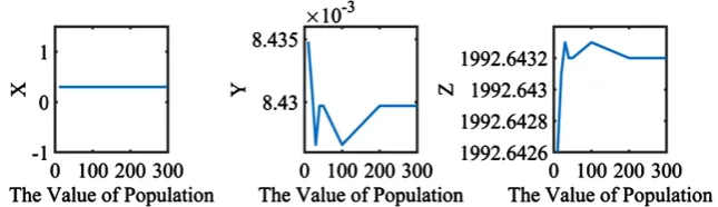
From the first graph of Figure 6, we can see that as the value of population increases, the value of X does not change significantly, and the form of the curve seems to be a straight line, indicating that population does not have much influ-ence on the value of X. As can be seen from the second graph of Figure 6, al-though there are fluctuations in the graph, the change of value is small, and it can be considered that there is not much correlation between Y and population. From the third graph of Figure 6, we can see that if we only observe from the curve, we will find that with the increase of the population value, the value of Z
in the first half will rise sharply, and then gradually converge to the optimal so-lution. But if only measured by the magnitude of the value, it can be seen that there is not much change in the value of Z, indicating that the value of popula-tion does not have much influence on the parameter of optimizapopula-tion.
From the first graph of Figure 7, it can be seen that as the binary length of the variable increases, the value of X hardly changes. According to the previous re-sult, it can be seen that X converges to optimal resolution. From the second graph of Figure 7, it can be seen that as the binary length of the variables in-creases, the value of Y increases sharply at the beginning and gradually con-verges to a certain value after a short period of fluctuation. From the third graph of Figure 7, it can be seen that as the binary length of the variable increases, Z
increases. The value of the rapid increase in the first half part, and then tends to be stable, indicating that by increasing the binary length of the variables, we can obtain optimal solution to get the maximum benefit.
5. Simulated Annealing Algorithm
5.1. The Principle of Simulated Annealing Algorithm
DOI: 10.4236/jamp.2018.66102 1225 Journal of Applied Mathematics and Physics
Figure 6.The effects of population on quantum genetic algorithm.
Figure 7.The effects of the length of variables on quantum genetic algorithm.
and a control parameter called temperature. As typically implemented, the si-mulated annealing approach involves a pair of nested loops and two additional parameters, a cooling ratio and an integer temperature length. The probability that an uphill move of size will be accepted diminishes as the temperature de-clines, and for a fixed temperature, small uphill moves have higher probabilities of acceptance than large ones. This particular method of operation is motivated by a physical analogy, best described in terms of the physics of crystal growth [21]. Note that simulated annealing first builds up a rough view of the surface by moving with large step lengths. As the temperature falls and the step length de-creases, it slowly focuses on the most promising area. In this way, the algorithm can escape from local maxima through downhill moves. Eventually, the algo-rithm should converge to the function’s global maximum [22].
5.2. The Process of Simulated Annealing Algorithm
DOI: 10.4236/jamp.2018.66102 1226 Journal of Applied Mathematics and Physics that the SA accepts the new solution. For the optimization of objective function, the probability that SA accepts new solution is based on principle. After that, determine the relationship between current solution and new solution, and termine the relationship between the two based on the equations in order to de-termine whether the new solution should be accepted or rejected. Repeating the following process can see that the temperature at the beginning is very high, and the probability that the SA accepts poor solutions is relatively high. This gives SA a greater chance of jumping out of local optimal solution. As the temperature gradually decreases, the probability of SA receiving a poor solution becomes smaller.
5.3. The Results of Simulated Annealing Algorithm
Simulated annealing algorithm is an important optimization method. The main factors affecting this algorithm are the number of iterations, max stall iterations, initial temperature, and anneal interval. This article discusses the influence of these four factors on optimization results, focusing on analyzing the influence of these factors on X, Y, and Z, and then determining the maximum benefit of pipelines.
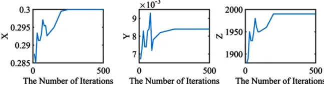
From the first graph of Figure 8, we can see that with the increase of the number of iterations, the trend of X increases, but there will be some fluctua-tions, and finally converge to a stable value. Compared with the previous results, at this time, the value of X will reach optimal solution. From the second graph of Figure 8, it can be seen that in initial stage, the value of Y fluctuates greatly, but gradually stabilizes to a certain value as the number of iterations continue to in-crease. The values are verified that Y will converge to the optimal solution. From the third graph of Figure 8, it can be seen from the overall trend of the curve that as the number of iterations increases, the value of Z fluctuates in the first half part and then turns to a certain stable value, indicating that by increasing the number of iterations can obtain the optimal solution and the maximum ben-efits.
[image:12.595.210.534.621.708.2]From the first graph of Figure 9, it can be seen that as the max stall iterations increase, the value of X rises sharply at first and then gradually becomes stable. From the second graph of Figure 9, it can be seen that with the increase of max stall iterations, the value of Y decreases rapidly at the initial stage and then tends to optimal solution. From the third graph of Figure 9, it can be seen that with
DOI: 10.4236/jamp.2018.66102 1227 Journal of Applied Mathematics and Physics
Figure 9.The effects of max stall iterations on simulated annealing.
the increase of max stall iterations, the value of Z rises rapidly in the initial stage and then tends to be stable. The optimal solution to the convergence shows that the maximum value can be obtained by increasing max stall iterations in order to obtain maximum benefits.
Another two factors that affect simulated annealing algorithm are initial tem-perature and annealing interval. After determining the number of iterations and max stall iterations, different values of effects on the values of X, Y, and Z were compared and analyzed. After the analysis is completed, it can be seen that these two factors do not have much influence on the optimization performance. Therefore, if you want to get the best solution and get the maximum benefits, you mainly need to determine the first two factors.
6. Conclusion
DOI: 10.4236/jamp.2018.66102 1228 Journal of Applied Mathematics and Physics parameters that need to be optimized in the quantum genetic algorithm. For this reason, this paper continues to apply simulated annealing algorithm to solve the optimization problem. It can be found that compared with the quantum genetic algorithm, the simulated annealing algorithm needs to determine fewer parame-ters, and it is not easy to fall into local extremes, and the performance is more stable. Therefore, this paper recommends simulated annealing algorithm to op-timize the construction and operation management of pipelines in order to ob-tain maximum profits.
References
[1] Chirehdast, M. and Ambo, S.D. (1995) Topology Optimization of Planar Cross-Sections. Structural Optimization, 9, 266-268.
https://doi.org/10.1007/BF01743982
[2] Liu, S., An, X. and Jia, H. (2008) Topology Optimization of Beam Cross-Section Considering Warping Deformation. Structural & Multidisciplinary Optimization, 35, 403-411.https://doi.org/10.1007/s00158-007-0138-y
[3] Ren, Y., Xiang, J., Lin, Z. and Zhang, T. (2016) A Novel Topology Optimization Method for Composite Beams. Proceedings of the Institution of Mechanical Engi-neers Part G Journal of Aerospace Engineering, 230, 1153-1163.
https://doi.org/10.1177/0954410015605547
[4] Blasques, J.P. and Stolpe, M. (2012) Multi-Material Topology Optimization of la-minated Composite Beam Cross Sections. Composite Structures, 94, 3278-3289.
https://doi.org/10.1016/j.compstruct.2012.05.002
[5] Griffiths, D.R. and Miles, J.C. (2003) Determining the Optimal Cross-Section of Beams. Advanced Engineering Informatics, 17, 59-76.
https://doi.org/10.1016/S1474-0346(03)00039-9
[6] Yoshimura, M., Nishiwaki, S. and Izui, K. (2005) A Multiple Cross-Sectional Shape Optimization Method for Automotive Body Frames. Journal of Mechanical Design, 127, 49-57.https://doi.org/10.1115/1.1814391
[7] Fontán, A.N., Hernández, S. and Baldomir, A. (2014) Simultaneous Cross Section and Launching Nose Optimization of Incrementally Launched Bridges. Journal of Bridge Engineering, 19, Article ID: 04013002.
https://doi.org/10.1061/(ASCE)BE.1943-5592.0000523
[8] Guerra, A. and Kiousis, P.D. (2006) Design Optimization of Reinforced Concrete Structures. Computers & Concrete, 3, 313-334.
https://doi.org/10.12989/cac.2006.3.5.313
[9] Cardoso, J.B. (2011) Cross-Section Optimal Design of Composite Laminated Thin-Walled Beams. Pergamon Press, Inc., Elmsford, NY.
[10] Muthukumaran, V., Rajmurugan, R. and Ram Kumar, V.K. (2014) Cantilever Beam and Torsion Rod Design Optimization Using Genetic Algorithm. International Journal of Innovative Research in Science, Engineering and Technology, 3, 2682-2690.
[11] Liu, Q., Paavola, J. and Zhang, J. (2016) Shape and Cross-Section Optimization of Plane Trusses Subjected to Earthquake Excitation Using Gradient and Hessian Ma-trix Calculations. Mechanics of Composite Materials & Structures, 23, 156-169.
https://doi.org/10.1080/15376494.2014.949921
DOI: 10.4236/jamp.2018.66102 1229 Journal of Applied Mathematics and Physics
Section by Employing Extrusion Constraint. American Institute of Physics, 1233, 964-969.https://doi.org/10.1063/1.3452311
[13] Zhang, Y., Hou, Y. and Liu, S. (2014) A New Method of Discrete Optimization for Cross-Section Selection of Truss Structures. Engineering Optimization, 46, 1052-1073.https://doi.org/10.1080/0305215X.2013.827671
[14] Mitchell, M. (1998) An Introduction to Genetic Algorithms. MIT Press, Cambridge. [15] Chen, L., Peng, J., Zhang, B. and Rosyida, I. (2017) Diversified Models for Portfolio Selection Based on Uncertain Semivariance. International Journal of Systems Science, 48, 637-648.https://doi.org/10.1080/00207721.2016.1206985
[16] Whitley, D. (1994) A Genetic Algorithm Tutorial. Statistics and Computing, 4, 65-85.https://doi.org/10.1007/BF00175354
[17] Zhang, B., Peng, J., Li, S. and Chen, L. (2016) Fixed Charge Solid Transportation Problem in Uncertain Environment and Its Algorithm. Computers & Industrial En-gineering, 102, 186-197.https://doi.org/10.1016/j.cie.2016.10.030
[18] Han, K.H. and Kim, J.H. (2000) Genetic Quantum Algorithm and Its Application to Combinatorial Optimization Problem. Proceedings of the 2000 Congress on Evolu-tionary Computation, La Jolla, 16-19 July 2000, 1354-1360.
[19] Laboudi, Z. and Chikhi, S. (2012) Comparison of Genetic Algorithm and Quantum Genetic Algorithm. International Arab Journal of Information Technology, 9, 243-249.
[20] Nowotniak, R. and Kucharski, J. (2010) Building Blocks Propagation in Quan-tum-Inspired Genetic Algorithm.
[21] Johnson, D.S., Aragon, C.R., Mcgeoch, L.A. and Schevon, C. (1989) Optimization by Simulated Annealing: An Experimental Evaluation. Part I, Graph Partitioning.
Operations Research, 37, 865-892.https://doi.org/10.1287/opre.37.6.865