Stellar Distance and Velocity

ISSN Online: 2327-4379 ISSN Print: 2327-4352

DOI: 10.4236/jamp.2019.71016 Jan. 25, 2019 181 Journal of Applied Mathematics and Physics

Stellar Distance and Velocity

Miloš Čojanović

Independent Scholar, Montreal, Canada

Abstract

In this paper, a method is presented by which it is possible to determine a distance between the sun and a star as well as a velocity at which the star moves relative to the sun. In order to achieve this, it is sufficient to know three positions of the star and the unit vectors determined by the star and three arbitrarily chosen points that do not lie on a single line. The method has been tested using the data generated by a computer program as well as real data ob-tained by Gaia mission. In the first case, we found the huge differences com-paring the results derived by the method to the results calculated by the tradi-tional parallax method. In the second case also, there are large differences be-tween the obtained and the expected results, but primarily because of the form of the input data, that is not fully suited to the proposed method. Under certain conditions, one would be able to find a velocity at which the sun is moving re-garding a stationary coordinate system (K) that will be defined later on.

Keywords

Stellar Distance, Stellar Velocity

1. Introduction

Stellar parallax is defined as an apparent change in position of a star against the background of more distant objects, due to the movement of the earth revolving around the sun. In order to calculate a distance to the star, it is enough to know a distance from the earth to the sun that serves as a base line and the parallax angle that is obtained by two the measurements that have been made six months apart. There are some shortcomings of this method. Firstly, the base line is fixed thus the angles measured are always extremely small. Secondly, the base line is directly affected by the movement of the sun but it is not taken into the consid-eration. Thirdly, during the time of six months, a star is moving and changing its position which also affects a parallax angle. In some cases, a parallax has a nega-tive value. It is believed that it may arise when the true parallax is smaller than How to cite this paper: Čojanović, M.

(2019) Stellar Distance and Velocity. Jour-nal of Applied Mathematics and Physics, 7, 181-209.

https://doi.org/10.4236/jamp.2019.71016

Received: December 11, 2018 Accepted: January 22, 2019 Published: January 25, 2019

Copyright © 2019 by author(s) and Scientific Research Publishing Inc. This work is licensed under the Creative Commons Attribution International License (CC BY 4.0).

http://creativecommons.org/licenses/by/4.0/

DOI: 10.4236/jamp.2019.71016 182 Journal of Applied Mathematics and Physics

its error. This assumption can only be partially correct, because some large nega-tive parallaxes have been measured. In this novel method, sun and star move-ments regarding the stationary frame (K) are taken into the calculation, which in certain cases could cause a negative parallax. The base line becomes a “base tri-angle” and its size is limited only by the time between the two measurements.

2. Conversion Spherical Coordinates into Cartesian

Coordinates

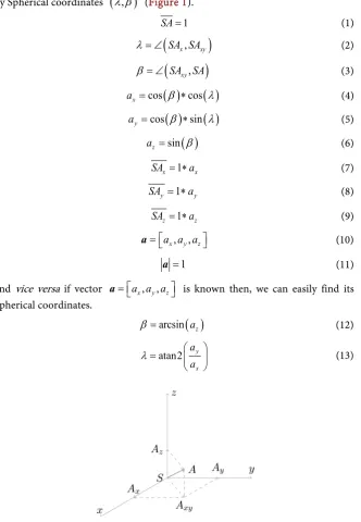
First we will derive well known formulas for transformation from Spherical into Cartesian coordinate system and vice versa. Let suppose that a point A is given by Spherical coordinates

(

λ β

,

)

(Figure 1).

1

SA= ₍₁₎

(

SA SAx, xy

)

λ

= ∠

(2)

(

SA SAxy,

)

β

= ∠

(3)

( )

( )

cos cos

x

a =

β

∗

λ

(4)

( )

( )

cos sin

y

a =

β

∗

λ

(5)

( )

sin

z

a =

β

(6) 1

x x

SA = ∗a ₍₇₎

1

y y

SA = ∗a

(8) 1

z z

SA = ∗a ₍₉₎

, ,

x y z

a a a

 

=  

a

(10) 1

=

a

₍₁₁₎

and vice versa if vector a= a a ax, ,y z is known then, we can easily find its

Spherical coordinates.

( )

arcsin az

β

=

(12)

atan2 y x a a λ=  

[image:2.595.212.545.229.710.2]

 

(13)

DOI: 10.4236/jamp.2019.71016 183 Journal of Applied Mathematics and Physics

3. The Heliocentric-Ecliptic Coordinate System

Let the S x y z

(

, ,

)

represents “The Heliocentric-Ecliptic Coordinate System” (Figure 2). Its origin S is at the center of the sun and the fundamental plane

( )

,

S x y coincides with the “ecliptic”, plane of the Earth’s revolution about the sun. On the first day of Spring a line joining the center of the Earth and the cen-ter of the sun points in the direction of positive x-axis. This is called a vernal equinox direction.

The use of The Heliocentric-Ecliptic Coordinate System is obsolete, but in present paper we will use it for a better explanation of the proposed method.

Direction SX0 represents Vernal equinox, and t1 the time needed the

Earth to move from the point X0 to the point A. We can say that (Figure 2)

depicts classical explanation how Earth revolves about the sun.

Now we will present a different interpretation of the same event. A stationary coordinate system marked as well by (K) is joined to this referential frame. The coordinate system (K) is not moving but rather remains fixed with respect to distant objects while the sun is moving by some velocity v (Figure 3) regard-ing the coordinate system (K).

In astronomy, an epoch is a moment in time used as a reference point, so we need to specify a certain time T0 (TT-Terrestrial Time), which we are using as a

[image:3.595.277.473.401.536.2]

reference. In other words an epoch is a moment for when a given position of an astronomical object is valid.

[image:3.595.211.542.567.694.2]

Figure 2. The position of the Earth in case the Sun is stationary regarding the (K).

DOI: 10.4236/jamp.2019.71016 184 Journal of Applied Mathematics and Physics

Finally we can suppose that for a certain period of time, a set of distant objects, the coordinate system (K) and Epoch uniquely determine Stationary Reference Frame (K). From Figure 2, it follows

149597870.7 km

AU= ₍₁₄₎

R AU=

₍₁₅₎

0

SA =R

₍₁₆₎

365.25 24 60 60

yearsec= × × ×

₍₁₇₎

1 1 0

t T T= −

₍₁₈₎

1

2 cos

x

t

A R

yearsec

 Π ∗ 

= ∗ _{ }

 

(19)

1

2 sin

y

t

A R

yearsec

 Π ∗ 

= ∗ _{ }

 

(20)

From Figure 3, it follows

, ,

x y z

v v v

 

=  

v

(21)

1 1 0

t T T= −

(22)

1

x x

S′ = ∗t v

(23)

1

y y

S′ = ∗t v

(24)

1

z z

S′ = ∗t v

(25)

1 1 cos 2

x x t

A t v R

yearsec

 Π ∗ 

= ∗ + ∗ _{ }

 

(26)

1 1 sin 2

y y t

A t v R

yearsec

 Π ∗ 

= ∗ + ∗ _{ }

 

(27)

1

z z

A = ∗t v

(28)

(

, ,

)

x x x y z

A = A v v v

(29)

(

, ,

)

y y x y z

A = A v v v

(30)

(

, ,

)

z z x y z

A =A v v v

(31) where T1 (TT time) is expressed in seconds

Thus we have got the coordinates for the center of the Earth (marked by A) regarding the (K). Assuming that the time t1 is known from Equations (29)-(31)

it follows that the coordinates of point A can be expressed as a function of the velocity v. For now v has been considered as a varible.

The astrometric processing uses a coordinate system known as the Barycentric Coordinate Reference System. It has its origin at the solar-system barycentre. Its axes are non-rotating with respect to objects at cosmological distances and coin-cide with those of the International Celestial Reference Frame.

The positions and proper motions of non-solar system objects derived from

DOI: 10.4236/jamp.2019.71016 185 Journal of Applied Mathematics and Physics

4. Coordinate Transformations

The basis vectors in the equatorial system are here denoted

[

x y z, ,

]

, The basis vectors in the ecliptic and galactic systems are respectively denoted

[

x y zk, ,k k

]

and x y zg, ,g g. Thus, the arbitrary direction u may be written in terms of the

equatorial, ecliptic and galactic coordinates in the following way [2].

The transformation between the equatorial and ecliptic systems is given by:

[

x y zk, ,k k

] [

= x y z AK, ,

]

∗

and

[

_{, ,}

]

[

_{, ,}

]

T

k k k

x y z = x y z ∗AK

where

23.4392911

obliquity= _{(J2000.0 degrees)}

π

1 0.409092802283074

180

obliquity obliquity = ∗ =

(

)

(

)

(

)

(

)

1 0 0

0 cos 1 sin 1

0 sin 1 cos 1

1 0 0

0 0.917482062146320 0.397777155753990 0 0.397777155753990 0.9174820621463209

AK obliquity obliquity

obliquity obliquity

 

 

=_ − _

 

 

 

 

=_ − _

 

 

(32)

1 T

1 0 0

0 0.917482062146320 0.397777155753990 0 0.397777155753990 0.9174820621463209

AK− AK

 

 

= _{=  }

 − 

 

(33)

The transformation between the equatorial and galactic systems is given by:

[

]

, , , ,

g g g

x y z x y z AG

  = ∗

 

where:

0.0548755604 0.4941094279 0.8676661490 0.8734370902 0.4448296300 0.1980763734 0.4838350155 0.7469822445 0.4559837762

AG

− + −

 

 

= −_ − − _

− + + 

 

(34)

1 T

0.0548755604 0.8734370902 0.4838350155 0.4941094279 0.4448296300 0.7469822445 0.8676661490 0.1980763734 0.4559837762

AG− AG

− − −

 

 

= = +_ − + _

− − + 

 

(35)

The transformation between the galactic and ecliptic systems is given by:

[

_{, ,}

]

_{, ,} 1 _{, ,} T_*

k k k g g g g g g

x y z _=x y z _∗AG− _∗AK_=x y z _∗AG AK

   

[

, ,

]

, ,

0.0548755604 0.9938213789915562 0.09647662628973946

0.4941094279 0.1109907336202431 0.8622858750870472

0.867666149 3.515899626965191 10 4 0.4971471917263599

k k k g g g

x y z x y z

E

 

=  

− − −

 

 

∗_ − _

− − − 

 

DOI: 10.4236/jamp.2019.71016 186 Journal of Applied Mathematics and Physics

The peculiar motion of the Sun [3] with respect to the LSR is

(

U V W, ,

)

=

[

11.1,12.24,7.25 km s

]

(

)

The velocity of the LSR about the center of the Milky Way is about 220 (km/sec), thus Sun velocity in Galactic coordinates is given by following equa-tion

[

11.1,232.24,7.25

]

g=

v ₍₃₇₎

Sun velocity in Ecliptic coordinates regarding the frame (K)

[

107.85, 36.81,202.79

]

k = −

v ₍₃₈₎

Of course, this can not be taken as a fully accurate value.

5. Determining a Distance to a Star and Its Velocity

regarding the Coordinate System (

K

)

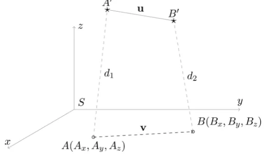
We assume that a star is moving with a uniform, rectilinear space motion u

relative to the referential frame (K). At the some momemt T (that will be derived later on) a signal has been emitted from the star (Figure 4). Postion of the star is marked by A′_{. At the instant t (Terrestrial Time) the signal has been recevied at} the point A on the Earth. Now we measure right ascension (

α

_{) and declination}

(

δ

) of the star regarding the equatorial coordinate system and transform them into the ecliptic longitude and ecliptic latitude

(

λ β

1, 1

)

that can be also

ex-pressed as a unit vector a= a a ax, ,y y regarding the coordinate system (K).

In this way the direction in which the star lies has been determined. In order to find a position (in pollar coordinates) of the star at the moment t we need to de-termine a distance between points A and A′_.

Analogously we have the similiar situation with the pairs of points

(

B B, ′

)

and

(

C C, ′

)

_{. Note that the points A B}′ ′_{, and} C′ _{are collinear while the} points A, B and C form a triangle.

1

d =AA′ ₍₃₉₎

2

[image:6.595.253.487.495.692.2]

d =BB′ ₍₄₀₎

DOI: 10.4236/jamp.2019.71016 187 Journal of Applied Mathematics and Physics 3

d =CC′ ₍₄₁₎

, ,

x y z

a a a

 

=  

a

(42)

( )

1

( )

1

cos cos

x

a =

β

∗

λ

(43)

( )

1

( )

1

cos sin

y

a =

β

∗

λ

(44)

( )

1

sin

z

a =

β

(45) , ,

x y z

b b b

 

=  

b (46)

( )

2

( )

2

cos cos

x

b =

β

∗

λ

(47)

( )

2

( )

2

cos sin

y

b =

β

∗

λ

(48)

( )

2

sin

z

b =

β

(49) , ,

x y z

c c c

 

=  

c

(50)

( )

3

( )

3

cos cos

x

c =

β

∗

λ

(51)

( )

3

( )

3

cos sin

y

c =

β

∗

λ

(52)

( )

3

sin

z

c =

β

₍₅₃₎

(

x, ,y z

)

A= A A A

(54)

1 1

2 cos

x x t

A t v R

yearsec

 Π ∗ 

= ∗ + ∗ _{ }

  (55)

1 1 sin 2

y y t

A t v R

yearsec

 Π ∗ 

= ∗ + ∗ _{ }

  (56)

1

z z

A = ∗t v

₍₅₇₎

(

x, ,y z

)

B= B B B

(58)

2 2

2 cos

x x t

B t v R

yearsec

 Π ∗ 

= ∗ + ∗ _{ }

  (59)

2 2 sin 2

y y t

B t v R

yearsec

 Π ∗ 

= ∗ + ∗ _{ }

  (60)

2

z z

B = ∗t v

₍₆₁₎

(

x, ,y z

)

C= C C C

(62)

3 3 cos 2

x x t

C t v R

yearsec

Π ∗

 

= ∗ + ∗ _{ }

  (63)

3 3 2 sin y y t

C t v R

yearsec

Π ∗

 

= ∗ + ∗ _{ }

  (64)

3

z z

C = ∗t v

₍₆₅₎

(

x, ,y z

)

A′= A A A′ ′ ′

(66)

1

x x x

A′ =A a d+ ∗ ₍₆₇₎

1

y y y

DOI: 10.4236/jamp.2019.71016 188 Journal of Applied Mathematics and Physics 1

z z z

A′ =A a d+ ∗ ₍₆₉₎

(

x, ,y z

)

B′= B B B′ ′ ′

(70)

2

x x x

B′ =B b d+ ∗

₍₇₁₎

2

y y y

B′ =B +b d∗ ₍₇₂₎

2

z z z

B′ =B b d+ ∗ ₍₇₃₎

(

x, ,y z

)

C′= C C C′ ′ ′

(74)

3

x x x

C′ =C + ∗c d ₍₇₅₎

3

y y y

C′ =C +c d∗ ₍₇₆₎

3

z z z

C′ =C c d+ ∗ ₍₇₇₎ The points A B′ ′, _and C′ _{are collinear therefore we can write a following} expression.

k

′ ′= ∗ ′ ′

A C A B

₍₇₈₎

where k is for now an unknown coefficient.

, ,

x x y y z z

A C A C A C

′ ′_{= } ′ ′ ′ ′ ′ ′_ A C

(79)

, ,

x x y y z z

A B A B A B

′ ′_{= } ′ ′ ′ ′ ′ ′_

A B

(80)

3 1, 3 1, 3 1

x x x x y y y y z z z z

C c d A a d C c d A a d C c d A a d

 + ∗ − − ∗ + ∗ − − ∗ + ∗ − − ∗ =

  (81)

2 1, 2 1, 2 1

x x x x y y y y z z z z

k B b d∗_ + ∗ −A a d B b d− ∗ + ∗ −A a d B b d− ∗ + ∗ −A a d− ∗ _(82)

(

k− ∗ ∗ − ∗ ∗ + ∗1

)

a d k b d c dx 1 x 2 x 3= − ∗

(

1 k A k B C

)

x+ ∗ x− x ₍₈₃₎

(

k− ∗ ∗ − ∗ ∗1

)

a d k b d c dy 1 y 2+ ∗y 3= − ∗

(

1 k A k B C

)

y+ ∗ y− y ₍₈₄₎

(

k− ∗ ∗ − ∗ ∗ + ∗1

)

a d k b d c dz 1 z 2 z 3= − ∗

(

1 k A k B C

)

z + ∗ z − z ₍₈₅₎

(

)

(

)

(

)

(

)

(

)

(

)

1 2 3 1 1 1 1 1 1

x x x x x x

y y y y y y

z z z z z z

k a k b c d k A k B C

k a k b c d k A k B C

k a k b c d k A k B C

− ∗ − ∗ − ∗ + ∗ −       _{− ∗ − ∗}  ₌ _{− ∗ + ∗ −}        − ∗ − ∗  _{ }  − ∗ + ∗ −      (86)

(

)

(

)

(

)

1 1 1

x x x

y y y

z z z

k a k b c

D k a k b c

k a k b c

− ∗ − ∗     =_ − ∗ − ∗ _  − ∗ − ∗    (87) 0

x x x

y y y

z z z

a b c

D a b c

a b c

    =       (88)

(

)

(

)

(

)

1 1 1

x x x

y y y

z z z

k A k B C

E k A k B C

k A k B C

− ∗ + ∗ −     =_ − ∗ + ∗ − _  − ∗ + ∗ −   

(89)

( )

det D ∆ = (90)

( )

0 det D0

∆ =

DOI: 10.4236/jamp.2019.71016 189 Journal of Applied Mathematics and Physics

( ) (

k k 1

)

0

∆ = − ∗ − ∗ ∆ (92)

(

)

(

)

(

)

1 1 1 1

x x x x x

y y y y y

z z z z z

k A k B C k b c

D k A k B C k b c

k A k B C k b c

− ∗ + ∗ − − ∗     =_ − ∗ + ∗ − − ∗ _  _{− ∗ + ∗ − − ∗}   

(93)

(

)

(

)

(

)

(

)

(

)

(

)

2 1 1 1 1 1 1

x x x x x

y y y y y

z z z z z

k a k A k B C c

D k a k A k B C c

k a k A k B C c

− ∗ − ∗ + ∗ −     =_ − ∗ − ∗ + ∗ − _  − ∗ − ∗ + ∗ −    (94)

(

)

(

)

(

)

(

)

(

)

(

)

3 1 1 1 1 1 1

x x x x x

y y y y y

z z z z z

k a k b k A k B C

D k a k b k A k B C

k a k b k A k B C

− ∗ − ∗ − ∗ + ∗ −     =_ − ∗ − ∗ − ∗ + ∗ − _  − ∗ − ∗ − ∗ + ∗ −    (95)

If

(

∆ ≠0

)

⇔ ∆ ≠

(

(

0 0

)

and

(

k≠0

)

and

(

k≠1

)

)

then we have

(

)

1

( )

_{( )}

1

1

det , , ,

det

x y z D

d k v v v

D

∆

= =

∆

(96)

(

)

2

( )

_{( )}

2

2

det , , ,

det

x y z

D d k v v v

D

∆

= =

∆

(97)

(

)

3

( )

_{( )}

3

3

det , , ,

det

x y z

D d k v v v

D ∆ = = ∆ (98)

In order to calculate distances d d d1, ,2 3 we have to determine a coefficient k.

Let t1 denotes the time when signal is received at the point A. If T1 denotes

the time when the signal was being emitted from the star at the point A′ _we will have following equation

1

1 1 d

T t c

= −

(99) where c denotes the speed of light in the reference frame K.

Analogously for the points B and B′ _{we will have}

2

2 2 d

T t c

= −

(100) Now we have

2 1

1 2 1 2 1 d d

T T T t t

c c

∆ = − = − − +

(101)

2 1

1 1 d d

T t

c c

∆ = ∆ − +

(102)

2 1

1 d 1 d

T t

c c

∆ + = ∆ +

(103) If T3 denotes the time when the signal was being emitted from the star at the

point C′ _and t₃ denoted the time when the signal is received at the point C

we will have following equation

3 1

2 3 1 3 1 d d

T T T t t

c c

∆ = − = − − +

DOI: 10.4236/jamp.2019.71016 190 Journal of Applied Mathematics and Physics

3 1

2 2 d d

T t c c ∆ = ∆ − + (105) 3 1 2 2 d d T t c c ∆ + = ∆ + (106) If u denotes magnitude of the velocity u then from Equation (78) it follows

1

A B u′ ′ = ∗∆T ₍₁₀₇₎

2

A C u′ ′ = ∗∆T ₍₁₀₈₎

(

)

2 1

u∗ ∆ = ∗ ∗ ∆T k u T

(109)

2 1

T k T

∆ = ∗ ∆

₍₁₁₀₎

Combining equations (102), (105) and (110) it follows that

3 1 2 1

2 1

d d d d

t k t

c c c c

 

∆ − + = ∗ ∆ −_ + _

  (111)

(

)

1 1 2 3 1 2 0

d ∗ − −k d k d∗ + + ∆ ∗ ∗ − ∆ ∗ =t c k t c

(112)

(

)

3

1 2

1 2

1 0

k k ∆ t c k t c

∆ ∆

∗ − − ∗ + + ∆ ∗ ∗ − ∆ ∗ =

∆ ∆ ∆ (113)

(

)

2

(

)

(

)

1 k 1 2 k 3 0 t c k1 k 1 0 t c k k2 1 0

∆ ∗ − − ∆ ∗ + ∆ − ∆ ∗ ∆ ∗ ∗ ∗ − + ∆ ∗ ∆ ∗ ∗ ∗ − = (114)

Dividing Equation (114) by k k∗ −

(

1

)

_{we obtain that}

(

3

)

1 2

0 1 0 2 0

1 1 t c k t c

k k k k

∆ ∆ ∆ − + − ∆ ∗ ∆ ∗ ∗ + ∆ ∗ ∆ ∗ = − ∗ − (115)

(

)

(

)

(

)

1 1 1 1

x x x x x

y y y y y

z z z z z

k A k B C k b c k A k B C k b c k A k B C k b c

− ∗ + ∗ − − ∗

∆ = − ∗ + ∗ − − ∗ =

− ∗ + ∗ − − ∗

(116)

(

₁

)

( )

2

x x x x x x x x x

y y y y y y y y y

z z z z z z z z z

A b c B b c C b c

A b c k k B b c k C b c k

A b c B b c C b c

∗ − ∗ + ∗ − + ∗ (117)

(

)

( )

2

1 11 k 1 k 12 k 13 k

∆ = ∆ ∗ − ∗ + ∆ ∗ − + ∆ ∗

(118)

(

)

( )

1

11 k 1 12 k 13

k

∆ _{= ∆ ∗ − + ∆ ∗ − + ∆}

(119)

(

)

(

)

1

11 12 k 13 11

k

∆ _{= ∆ − ∆ ∗ + ∆ − ∆}

(120)

1

1 1

x x x x x x x x

y y y y y y y y

z z z z z z z z

A B b c C A b c

A B b c k C A b c p k q

k _{A B b c C A b c}

− − ∆ _{= − ∗ + − = ∗ +} − − (121)

(

)

(

)

(

)

(

)

(

)

(

)

2 1 1 1 1 1 1

x x x x x

y y y y y

z z z z z

k a k A k B C c

k a k A k B C c

k a k A k B C c

− ∗ − ∗ + ∗ −

∆ = − ∗ − ∗ + ∗ − =

− ∗ − ∗ + ∗ −

DOI: 10.4236/jamp.2019.71016 191 Journal of Applied Mathematics and Physics

(

1

) (

1

)

(

1

)

(

1

)

x x x x x x x x x

y y y y y y y y y

z z z z z z z z z

a A c a B c a C c

a A c k k a B c k k a C c k

a A c a B c a C c

∗ − ∗ − + ∗ − + ∗ − (123)

(

) (

)

(

)

(

)

2 21 k 1 1 k 22 k k 1 23 1 k

∆ = ∆ ∗ − ∗ − + ∆ ∗ ∗ − + ∆ ∗ −

(124)

(

)

2

21 1 22 23

1 k k

k

∆ _{= ∆ ∗ − + ∆ ∗ − ∆}

−

(125)

(

)

(

)

2

22 21 21 23

1 k

k

∆ _{= ∆ − ∆ ∗ + ∆ − ∆}

− (126)

2

2 2

1

x x x x x x x x

y y y y y y y y

z z z z z z z z

a B A c a A C c

a B A c k a A C c p k q

k _{a B A c a A c c}

− −

∆

= − ∗ + − = ∗ +

−

− −

(127)

(

)

(

)

(

)

(

)

(

)

(

)

3

1 1

1 1

1 1

x x x x x

y y y y y

z z z z z

k a k b k A k B C

k a k b k A k B C

k a k b k A k B C

− ∗ − ∗ − ∗ + ∗ −

∆ = − ∗ − ∗ − ∗ + ∗ − =

− ∗ − ∗ − ∗ + ∗ −

(128)

(

₁

)

2

(

₁

) ( )

(

₁

)

x x x x x x x x x

y y y y y y y y y

z z z z z z z z z

a b A a b B a b C

a b A k k a b B k k k a b C k k

a b A a b B a b C

∗ − ∗ + ∗ − ∗ − ∗ + ∗ − ∗ (129)

(

)

2

(

)

2

(

)

3 31 k 1 k 32 k 1 k 33 k 1 k

∆ = ∆ ∗ − ∗ − ∆ ∗ − ∗ + ∆ ∗ − ∗

(130)

(

_{k 1}3

)

_k 31

(

k 1

)

32 k 33

∆

= ∆ ∗ − − ∆ ∗ + ∆

− ∗

(131)

(

_{k 1}3

)

_k

(

31 32

)

k

(

33 31

)

∆

= ∆ − ∆ ∗ + ∆ − ∆

− ∗ (132)

(

₁3

)

3 3

x x x x x x x x

y y y y y y y y

z z z z z z z z

a b A B a b C A

a b A B k a b C A p k q

k k _{a b A B a b C A}

− −

∆ _{= − ∗ + − = ∗ +}

− ∗

− −

(133)

And finally the Equation (115) can be written in the following form 0

A k B∗ + =

₍₁₃₄₎

1 2 3 1 0

A p p= − +p − ∆ ∗ ∗ ∆t c ₍₁₃₅₎

1 2 3 2 0

B q q= − +q + ∆ ∗ ∗ ∆t c ₍₁₃₆₎

(

, ,

)

(

₍

, ,

)

₎

, ,

x y z x y z

x y z

B v v v k v v v

A v v v

= −

(137)

If (A≠0) then the Equation (134) has a unique solution, therefore the Equa-tions (96)-(98) have unique solution, as well.

If A, B and C are collinear points, then it follows that

AC= ∗α AB

(138) It is easy to prove that k=

α

, what implies that matrix E=0. In that case we would have only a trivial solution d1 =d2 =d3 =0.

DOI: 10.4236/jamp.2019.71016 192 Journal of Applied Mathematics and Physics

1, ,2 3

d d d are expressed only as a function of v.

(

)

1 1 x, ,y z

d =d v v v

(139)

(

)

2 2 x, ,y z

d =d v v v

(140)

(

)

3 3 x, ,y z

d =d v v v

(141) We will see later how the change in the value of velocity v affects the dis-tances d d d1, ,2 3.

We assume that the coordinates of the points A B′ ′, _{and C}′ _and corres-ponding distances d d1, 2 and d3 are known thus we are able to determine a

velocity u of the star regarding the frame (K). We have got the following equa-tions.

, ,

x y z

u u u

 

=  

u

(142)

2

T

′ ′ =

∆ A C u

(143)

(

)

3 1

2

, , x x x x

x x y z C A c d a d

u v v v

T

− + ∗ − ∗

=

∆

(144)

(

)

3 1

2

, , y y y y

y x y z

C A c d a d

u v v v

T

− + ∗ − ∗

=

∆ (145)

(

)

3 1

2

, , z z z z

z x y z C A c d a d

u v v v

T

− + ∗ − ∗

=

∆

(146)

2 2 2

x y z

u u u

= + +

u

(147)

6. The Case When

v

= 0

In this section it will be considered a case when v is unknown. Unlike the unit vectors a b c, , that are obtained by measurements and remain unchanged, vec-tor v will be substituted by 0 and u by ∆u. Therefore the formulas given in the [Section 5] get the new forms.

0

x

v = ₍₁₄₈₎

0

y

v = ₍₁₄₉₎

0

z

v = ₍₁₅₀₎

(

A A Ax, ,y z

)

=

A (151)

1 1 0 cos 2

x

t

A t R

yearsec

 Π ∗ 

= ∗ + ∗ _{ }

 

(152)

1 1 0 sin 2

y t

A t R

yearsec

 Π ∗ 

= ∗ + ∗ _{ }

  (153)

1 0

z

A = ∗t ₍₁₅₄₎

(

B B Bx, ,y z

)

=

B

DOI: 10.4236/jamp.2019.71016 193 Journal of Applied Mathematics and Physics

2 2

2

0 cos

x t

B t R

yearsec

 Π ∗ 

= ∗ + ∗ _{ }

 

(156)

2 2 0 sin 2

y t

B t R

yearsec

 Π ∗ 

= ∗ + ∗ _{ }

 

(157)

2 0

z

B = ∗t

₍₁₅₈₎

(

C C Cx, ,y z

)

=

C (159)

3 3 0 cos 2

x t

C t R

yearsec

Π ∗

 

= ∗ + ∗ _{ }

  (160)

3 3

2

0 sin

y t

C t R

yearsec

Π ∗

 

= ∗ + ∗ _{ }

 

(161)

3 0

z

C = ∗t

₍₁₆₂₎

...Finally we have got

(

)

1 1 0,0,0

d ≈d

(163)

(

)

2 2 0,0,0

d ≈d

(164)

(

)

3 3 0,0,0

d ≈d

(165) ...and

3 1

2

x x x x

x C A c d a d

u

T

− + ∗ − ∗

∆ ≈

∆ (166)

3 1 2

y y y y

y

C A c d a d

u

T

− + ∗ − ∗

∆ ≈

∆ (167)

3 1

2

z z z z

z C A c d a d

u

T

− + ∗ − ∗

∆ ≈

∆ (168)

In that way we are able to determine approximate values for distances d d d1, ,2 3

and star velocity ∆u regarding the sun.

In the special case, instead of a star, we can observe the barycenter of the Ga-laxy. Then ∆u denotes the velocity at which the barycenter of the Galaxy “moves” relative to the sun. In other words vg = −∆u denotes the velocity at

which the Sun is moving about the barycenter of the Galaxy.

7. Determining a Position of a Star

In this section it will be explained how to find a position of the star at some in-stant t2 if the following elements are known:

• v velocity of the sun regarding the reference frame (K)

• u velocity of a star regarding the reference frame (K)

• _distance d₁ between the Earth and star at some instant t1

• _{spherical coordinates of the star at point A given by unit vector} a= a a ax, ,y z

at instant t1

Thus our goal is to find the position of the star B′=

(

B B Bx′ ′ ′, ,y z

)

at instant

2

[image:14.595.237.508.74.233.2]

DOI: 10.4236/jamp.2019.71016 194 Journal of Applied Mathematics and Physics

Figure 5. Two positions A′ _{and B}′ _{of the star and the corresponding positions A and}

B of the Earth

known.

Therefore we get following equations

1 2 1

t t t

∆ = − ₍₁₆₉₎

(

x, ,y z

)

A′= A A A′ ′ ′

(170)

1

x x x

A′ = A a d+ ∗ ₍₁₇₁₎

1

y y y

A′ =A +a d∗ ₍₁₇₂₎

1

z z z

A′ =A a d+ ∗ ₍₁₇₃₎

(

x, ,y z

)

B= B B B

(174)

1

x x x

B =A + ∆ ∗t v ₍₁₇₅₎

1

y y y

B =A + ∆ ∗t v

(176)

1

z z z

B =A + ∆ ∗t v ₍₁₇₇₎

(

x, ,y z

)

B′= B B B′ ′ ′

(178)

1

x x x

B′ =A′+ ∆ ∗T u ₍₁₇₉₎

1

y y y

B′ =A′+ ∆ ∗T u ₍₁₈₀₎

1

z z z

B′=A′+ ∆ ∗T u ₍₁₈₁₎

2 1 1 1

d ∗ =b BB′= −∆ ∗ + ∗ + ∆ ∗t v d a T u ₍₁₈₂₎

2 2 2 2 2 2

2 1 1 1 1 1

1 1 1 1

2

2 2

d t v d u T t d

t T d T

= ∆ ∗ + + ∗ ∆ − ∗ ∆ ∗ ∗ ∗

− ∗ ∆ ∗ ∗ ∗ ∆ + ∗ ∗ ∗ ∗ ∆

v a

v u a u (183)

Obviously ∆T1 represents the time it takes for the star to move from the

point A′ _{to the point B}′_{. On the other hand we have}

1 2

1 1

d _t d _T

c + ∆ = c + ∆ (184)

2 1 1 1

d =d c+ ∗ ∆ − ∗ ∆t c T ₍₁₈₅₎

2 2 2 2 2 2

2 1 1 1 1 1

2

1 1 1 1

2

2 2

d d c t c T d c t

d c T c t T

= + ∗ ∆ + ∗ ∆ + ∗ ∗ ∗ ∆

DOI: 10.4236/jamp.2019.71016 195 Journal of Applied Mathematics and Physics

From the Equations (183) and (186) we have

(

)

(

)

(

)

(

)

2 2 2 2

1 1 1 1 1 1 2 2 2

1 1 1

2

2 0

c u T d c c t t d T

c v t d t c

− ∆ − + ∆ − ∆ + ∆

+ − ∆ + ∆ + =

uv au

va (187)

The Equation (187) can be written in the following short form and solved by an unknown ∆T1

2 2

A c u= −

₍₁₈₈₎ 2

1 1 1 1

B d c c t= + ∆ − ∆tuv+dau ₍₁₈₉₎

(

2 2

)

2

(

)

1 2 1 1

C= c −v ∆ +t d t c∆ +va

(190)

2 _{2 0}

A x∗ − ∗ ∗ + =B x C ₍₁₉₁₎

2

1,2 B B A C

x

A

± − ∗

=

(192) There are two roots x1 and x2, but since d2 >0 it follows that

2 1 1

1 1 0 1 1

d d _{t T} d _{t T}

c c c

 _{= + ∆ − ∆ >} _⇒ _{+ ∆ > ∆} 

   

   

Thus we will choose a root of the Equation (191) for which this condition is fulfilled.

Now, when ∆T1 is known we are able to determine point B′, distance d2

and a unit vector b.

(

)

2

(

)

2

(

)

2

2 x x y y z z

d =BB′= B B′− + B B′− + B B′−

(193)

2

x x

x B B

b d

′ − =

(194)

2

y y

y

B B

b d

′ − =

(195)

2

z z

z

B B b

d

′ − =

(196) , ,

x y z

b b b

 

=  

b (197)

Now we will transform the unit vector a= a a ax, ,y z from ecliptic to

equatorial system. Transformed unit vector is marked by a eq_ .

T

_ =a a ax, ,y z∗AK

a eq (198)

[ ]

_ _ 1,1

x

a eq=a eq

₍₁₉₉₎

[ ]

_ _ 1,2

y

a eq=a eq

₍₂₀₀₎

[ ]

_ _ 1,3

z

a eq=a eq

₍₂₀₁₎

By transformation from a right-angle coordinate system into the spherical coordinates we obtain the following equations

1

_ atan2

_

y

x a eq a eq

α = _ _

DOI: 10.4236/jamp.2019.71016 196 Journal of Applied Mathematics and Physics

(

)

1 arcsin a eqz_

δ

=

(203) The same procedure will be repeated for unit vector b= b b bx, ,y z.

T

_ =b b bx, ,y z∗AK

b eq (204)

[ ]

_ _ 1,1

x

b eq=b eq

₍₂₀₅₎

[ ]

_ _ 1,2

y

b eq=b eq

₍₂₀₆₎

[ ]

_ _ 1,3

z

b eq=b eq

₍₂₀₇₎

2

_ atan2

_

y

x b eq b eq

α =  

  (208)

(

)

2 arcsin b eqz_

δ

= ₍₂₀₉₎

where coordinates

(

α δ

1, 1

)

and

(

α δ

2, 2

)

represent positions of the star in the

points A and B respectively.

We will define a proper motion (

µ

_{) as angular changes per year in the star’s}

right ascension (µRA) and declination (µDEC), using a constant epoch. Now we

will calculate proper motion components (µRA) and (µDEC).

Referring to (Figure 6) we get

1

SA SD SA SD′= ′= = = ₍₂₁₀₎

(

)

1 x SA,

α

= ∠ ′

(211)

(

)

2 x SD,

α

= ∠ ′

₍₂₁₂₎

(

)

2 1 A SD

α α α

′ ′

∆ = − = ∠

₍₂₁₃₎

(

)

(

)

1 A SA D SD

δ

= ∠ ′ = ∠ ′

(214)

S A SA′ _ ′

(215)

S D SD′  ′ ₍₂₁₆₎

(

,

)

RA SA SD

µ

= ∠

(217)

( )

1

( )

1

cos cos

S A S D SA′ = ′ = ∗

δ

=

δ

(218)

sin

2 2

AD S A

α

∆

 

= _{ }

′

[image:16.595.212.542.72.250.2]

∗   (219)

DOI: 10.4236/jamp.2019.71016 197 Journal of Applied Mathematics and Physics

( )

1

sin cos sin

2 2 2

AD S A_{= ′ ∗} ∆α_{= δ ∗} ∆α

   

   

(220)

( )

1

sin cos sin

2RA 2 2 2

AD AD

SA

µ _δ ∆α

 _{= = = ∗}  

 

  _{∗  }

  (221)

( )

1

2 arcsin cos sin 2

RA

α µ = ∗ _ δ ∗ _∆ __

 

  (222)

Since ∆

α

is a small angle it follows that

( )

1

( )

1

( )

1

arcsin cos sin cos sin cos

2 2 2

α α α

δ δ δ

 _∗ ∆ _{≈ ∗} ∆ _{≈ ∗}∆ 

 _ _ _ _ _ _

  (223)

( )

1

( ) (

1 2 1

)

cos cos

RA

µ

≈

δ

∗ ∆ =

α

δ

∗

α α

−

(224) It is trivial to prove that

2 1

DEC

µ =δ −δ ₍₂₂₅₎

or if we expressed them in milliarcseconds we get

[

mas

]

(

RA

) (

180 3600 1000

)

RA

µ

µ = × × ×

Π (226)

[

mas

]

(

DEC

) (

180 3600 1000

)

DEC

µ

µ = × × ×

Π (227)

8. The Second Part

In this section are given descriptions of four programs written in Maxima[4]. The purpose of their writing is testing the results obtained in the previous chap-ters. Instead of using the real measurements we will use data that are generated by a computer program. These data are presented in spherical coordinates

(

λ β

,

)

_{or as a corresponding unit vector} a= a a ax, ,y z regarding the

coor-dinate system (K). We assume that velocities v and u as well a distance d1

between the star and Earth at some instant t are known.

Since the distances between the sun and stars are expressed by large numbers, 64-bits floating-point format which gives from 15 to 17 significant decimal digits is not sufficient to make enough precise arithmetic operations. Therefore, for correct and precise testing, a quad precision (128-bit or 34-digit) is required.

Stellar parallax, proper motion and velocity

If the vectors b= b b bx, ,y z and c= c c cx, ,y z are respectively

corres-ponding unit vectors at points B and C [Figure 4] it is possible to calculate stel-lar parallax and its distance from the Earth using well known formulas. The time between two measurements is equal to six months.

AU is as usual defined as astronomical unit.

1 arccos 2

parallax= ∗ _ ⋅ _

⋅ ∗ ⋅

 

b c

b b c c

(228)

(

)

sin

AU distance

parallax

=

DOI: 10.4236/jamp.2019.71016 198 Journal of Applied Mathematics and Physics

Since we work with approximate values, instead of b =1 and c =1 we will rather use b = b b⋅ and c = c c⋅

Let suppose that we observe a star from our Galaxy which has a following spherical coordinate regarding the equatorial coordinate system [label=]

• RA 12.56=

• DEC= −57.81

These are field descriptions from the Table 1 and Table 2.

• v= v v vx, ,y z—sun velocity [km/sec]

• u= u u ux, ,y z—star velocity [km/sec]

• Real dist. —presumed distance between the star and Earth [Section 7] [km]

•

PRX

_{—parallax [Equation (228) [mas]]} • Dist PRX

(

)

—distance [Equation (229)] [km]

• Coeff —a ratio between the two distances, Coeff Dist PRX

(

)

Realdist

=

• PM RA. —proper motion (right ascension) [mas/year]

• PM DEC. —proper motion (declination) [mas/year]

By comparing the first and second rows, we can conclude that by changing only one component uz of the velocity u and keeping the values of all other

elements unchanged, parallax and proper motion have been drastically changed. By comparing first, second and third rows, we can conclude that despite the same distances, but due to the different values for velocity u, we obtain differ-ent values for the parallaxes. By comparing the first and fifth row, it follows that assuming that the sun is stationary, it does not significantly affect the value of the parallax nor the value of the proper motion.

[image:18.595.55.539.491.626.2]

It follows from the sixth row that when u=0 and v=0 it is possible di-rectly calculated the distance by means of parallax.

Table 1. Parallax and proper motion of the star.

x

v vy vz ux uy uz Real dist. PRX(mas) Dist PRX( ) Coeff PM.RA PM.DEC

1. 107.852 −36.81 202.79 vx+40 vy+50 vz+60 1.8 E15 78.81 3.91 E14 0.2175 214.70 233.63

2. 107.852 −36.81 202.79 vx+40 vy+50 vz−60 1.8 E15 7.6067 4.0565 E15 2.2536 46.187 −10.445

3. 107.852 −36.81 202.79 vx+80 vy+100 vz+120 1.8 E15 157.20 1.962 E14 0.109 429.416 467.27

4. 107.852 −36.81 202.79 vx+80 vy+100 vz+120 3.6 E15 78.57 3.92719 E14 0.109 214.7088 233.637

5. 0 0 0 40 50 60 1.8 E15 78.78 3.91672 E14 0.217595 214.7079 233.6343

6. 0 0 0 0 0 0 1.8 E14 171.426 1.800001 E14 1.00000055 −2.31E−9 1.4E−8

Table 2. Proper motion of the star during the period of the six months.

x

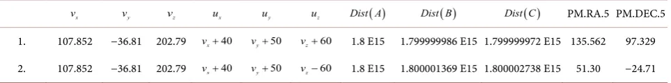
v vy vz ux uy uz Dist A( ) Dist B( ) Dist C( ) PM.RA.5 PM.DEC.5

1. 107.852 −36.81 202.79 vx+40 vy+50 vz+60 1.8 E15 1.799999986 E15 1.799999972 E15 135.562 97.329

[image:18.595.59.541.657.717.2]

DOI: 10.4236/jamp.2019.71016 199 Journal of Applied Mathematics and Physics

These are field descriptions from the Table 2.

• Dist A

( )

—distance from the point A to the star [km]

• Dist B

( )

—distance from the point B to the star [km]

• Dist C

( )

—distance from the point C to the star [km]

• PM RA. .5— proper motion (right ascension) [mas/(0.5*year)]

• DEC RA. .5—proper motion (declination) [mas/(0.5*year)]

Comparing the first row of the table T1 with the first row of the table T2, we can conclude that the angular motion of the star in a period of one year is roughly twice as large as its angular motion in six months. Comparing the second row of the Table T1 with the the second row of the Table T2, we can conclude that the angular motion of a star over a period of six months is greater than the one in one year. So in this case it would appear that the star is moving zigzag.

Motion toward or away from the Sun called radial velocity is determined by using the Doppler Effect. Motion perpendicular to the direction to the Sun is called tangential velocity. It is accepted that transverse velocity VT is given by a

following formula:

T

V = ∗ ∗k µ d ₍₂₃₀₎

where distance is noted by d, proper motion is noted by

µ

and the factor k

comes from the unit conversion.

We are going to test the correctness of this formula.

Let the vector v represents the velocity of the sun and the vector u represents the velocity of the star regarding the (K). Relative velocity ∆ = ∆u  ux,∆uy,∆uz

of the star regarding the sun is given by following equations.

∆ = −u u v

₍₂₃₁₎

x x x

u u v

∆ = −

₍₂₃₂₎

y y y

u u v

∆ = −

(233)

z z z

u u v

∆ = −

₍₂₃₄₎

Let us, regarding the coordinate system (K), define three unit vectors. The first vector noted by z radial_ is directed to the star. Therefore, its spherical coordinates are

(

λ β

,

)

, where

λ

represents ecliptic longitude and β repre- sents ecliptic latitude. The second one marked by x pmlong_ is determined by star proper motion in longitude direction. Its spherical coordinates are

(

λ

+π 2,0

)

_{. And the third one marked by} y pmlat_ will be determined by star proper motion in latitude direction. Its spherical coordinates are

(

λ β

, +π 2

)

_.

(

)

( )

( )

(

)

( )

_ =_cos

λ

+π 2 cos 0 ,cos 0 sin∗ ∗

λ

+π 2 ,sin 0 _

x pmlong (235)

( )

(

)

(

)

( )

(

)

_ =_cos

λ

∗cos

β

+π 2 ,cos

β

+π2 sin∗

λ

,sin

β

+π 2 _

y pmlat (236)

( )

( )

( )

( )

( )

_ =_cos

λ

∗cos

β

,cos

β

∗sin

λ

,sin

β

_

z radial

(237)

DOI: 10.4236/jamp.2019.71016 200 Journal of Applied Mathematics and Physics

at the center of the sun. We can find the scalar projections of the vector ∆u

onto the unit vectors z radial x pmlong_ , _ and y pmlat_ which is the same as to transform ∆u from the coordinate system (K) to the coordinate system (K’).

_ _

u long

∆ =x pmlong∗ ∆u ₍₂₃₈₎

_ _

u lat

∆ = y pmlat∗ ∆u

₍₂₃₉₎

_ _

u radial

∆ =z radial∗ ∆u ₍₂₄₀₎

Let define AZ a transformation matrix from coordinate system (K’) to the coordinate system (K) by the following equation.

(

)

( )

( )

(

)

( )

( )

(

)

(

)

( )

(

)

( )

( )

( )

( )

( )

cos π 2 cos 0 cos 0 sin π 2 sin 0

cos cos π 2 cos π 2 sin sin π 2

cos cos cos sin sin

AZ

λ λ

λ β β λ β

λ β β λ β

+ ∗ ∗ +

 

 

=_ ∗ + + ∗ + _

 ∗ ∗ 

 

(241)

( )

( )

( )

( )

( )

( )

( )

( )

( )

( )

( )

( )

sin cos 0

cos sin sin sin cos

cos cos cos sin sin

λ λ

λ β β λ β

λ β β λ β

−

 

 

= −_ ∗ − ∗ _

 ∗ ∗ 

 

(242)

By transforming the velocity ∆u from the coordinate system (K) to the coordinate system (K’), we obtain the following equation

[

_{∆u long u lat u radial_ , _ , _∆ ∆}

]

_{= ∆ ∗u AZ}T

(243)

(

)

2

tan .

_ d PM LONG

u pmlong

T

∗

∆ =

∆

(244)

(

)

2

tan .

_ d PM LAT

u pmlat

T

∗

∆ =

∆ (245)

where distance between the sun and a star is noted by d and ∆T2 is defined by

Equation (105).

If the formula given by the Equation (230) is valid then we should have that

_ _

u long u pmlong

∆ = ∆

₍₂₄₆₎

_ _

u lat u pmlat

∆ = ∆ ₍₂₄₇₎

From the two examples shown in Table 3, we can see that the conditions giv-en by (246) and (247) are met.

[image:20.595.227.539.232.330.2]

Matrix AZ is an orthogonal matrix. As a linear transformation, an orthogonal matrix preserves the dot product of vectors. In other words orthogonal transfor-mations preserve lengths of vectors and angles between them. Let PM LONG.

Table 3. Transverse velocity of a star determined in two ways.

x

u

∆ ∆u_y ∆u_z ∆u long_ ∆u lat_ ∆u radial_ _{Distance PM.LONG PM.LAT} ∆u pmlong_ ∆u pmlat_

1. 10 20 30 8.740 35.5236 −7.8528 1.8 E15 31.6001 128.4824 8.73817 35.52842