http://dx.doi.org/10.4236/jsea.2012.54028 Published Online April 2012 (http://www.SciRP.org/journal/jsea)
Lyapunov-Based Dynamic Neural Network for Adaptive
Control of Complex Systems
Farouk Zouari, Kamel Ben Saad, Mohamed Benrejeb
Unité de Recherche LARA Automatique, Ecole Nationale d’Ingénieurs de Tunis (ENIT), Tunis, Tunisia. Email: zouari.farouk@gmail.com, {kamel.bensaad, mohamed.benrejeb}@enit.rnu.tn
Received December 14th,2011; revised January 17th, 2012; accepted February 20th, 2012
ABSTRACT
In this paper, an adaptive neuro-control structure for complex dynamic system is proposed. A recurrent Neural Network is trained-off-line to learn the inverse dynamics of the system from the observation of the input-output data. The direct adaptive approach is performed after the training process is achieved. A Lyapunov-Base training algorithm is proposed and used to adjust on-line the network weights so that the neural model output follows the desired one. The simulation results obtained verify the effectiveness of the proposed control method.
Keywords: Complex Dynamical Systems; Lyapunov Approach; Recurrent Neural Networks; Adaptive Control
1. Introduction
For several decades, the problem of adaptive control of complex dynamic systems causes the interest of automa- tion specialists. The use of Proportional-Integral-Deriva- tive (PID) controllers is simple to perform, that give poor performance if there are uncertainties and nonlinearities in the system to be controlled. In several references like [1-3], neural networks are presented as tools to solve control problems due to their ability to model systems without analyzing them theoretically and their posses- sions a great capacity for generalization, which gives them a good robustness to noise [4].
Several strategies of the neural adaptive control exist which we quote: direct adaptive neural control, indirect adaptive neuronal control, adaptive neural internal model control, adaptive depth control based on feedforward ne- ural networks, robust adaptive neural control, Feedback- Linearization based neural adaptive control, adaptive ne- ural network model based nonlinear predictive control [5-13]. Each strategy has neural adaptive control archi- tecture, the algorithms used during the calculation of the parameters and stability conditions. It has three types of neural adaptive control architectures. The first type of architecture consists of a neural controller and a system to be controlled. The second type of neural architecture includes a controller, a system to be controlled and his neural model. The third type of architecture is composed of a neuronal controller, one or more robustness filter, a system to be controlled and his neural model.
The adjustment of the model parameters and the con-
troller is performed by neural learning algorithms that are based on the choice of the criterion to minimize, a mini- mization method and the theory of Lyapunov for stability and borniture of all signals existing. Several minimiza- tion methods exist which are presented: simple gradient method, gradient method with variable pitch, Newton method and Levenberg-Marquardt method [14].
The contribution of this paper is to propose an adap- tive Lyapunov-Based control strategy for complex dyna- mic system. The control structure takes advantage of Artificial Neural Network (ANN) learning and generali- zation capabilities to achieve accurate speed tracking and estimation. ANN-Based controllers lack stability proofs in many control structure applications and tuning them in a cascaded control structure is a difficult task to under- take. Therefore, we proposed a Lyapunov stability-Based adaptation technique as an alternative to the conventional gradient-Based and heuristic tuning methods. Thus, the stability of the proposed approach is guaranteed by Lya- punov Stability direct method unlike many computa- tional intelligence- Based controllers.
The different sections of this paper are organized as follows: in Section 2, we present the considered recurrent neural network and the proposed Lyapunov learning al- gorithm used for updating the weight parameters of the model system.
2. Neural Network Modeling Approach
Neural network modeling of a system from samples af- fected by noise usually requires three steps. The first step is the choice of neural network architecture, that is to say, the number of neurons in the input layer which is a func- tion of past values of the input and output, the number of hidden neurons, the number of neurons in the output layer neurons and the organization of them. The work [15,16] show that every continuous function can be ap- proximated by a neural network with three layers, the activation functions of neurons are respectively the sig- moid function for hidden layer neurons and linear func- tion for neurons in the output layer. There are two types of architectures of multilayer neural networks: neural networks, non-curly (static networks) and neural net- works curly or recurrent (dynamic networks). Neural net- works are non curly most used in the identification and control systems [17]. They may not be powerful enough to model complex dynamic systems with respect to neu- ral networks curly. Different types of recurrent neural networks have been proposed and have been successfully applied in many fields [18-25]. The structure of fully connected recurrent neural networks which was proposed by Williams and Zipser [26], is most often used [27,28] because of its generality. The second step is learning or in other words, estimating the parameters of the network from examples of input-output system identification. The methods of learning are numerous and depend on several factors, including the choice of error function, the initia- lization of weights, and the selection of the learning al- gorithm and the stopping criteria of learning. Learning strategies were presented in several research works that we cite [29-31]. The third step is the validation of the neural network obtained using the testing criteria for measuring performance. Most of these tests require a data set that was not used in learning. Such a test set or validation should, if possible, cover the same range of operation given that all learning.
2.1. Architecture of the Recurrent Neural Network
In this work, we consider a recurrent neural network (Figure 1) for identification of complex dynamic systems to a single input and single output. The architecture of these networks is composed of two parts: a linear model the linear behavior of the system and a non-linear ap- proach to nonlinear dynamics.
where:
ˆ y k u
is the output of the neural network at time k, and y are respectively the input and output system to identify,
1
1 1
x
x
e
f x
e
[image:2.595.326.519.87.178.2] and f2 x
Figure 1.Architecture of the considered neural network.
ctions of neurons,
h the number of neurons in the hidden layer respec-
tively of the model and controller,
n
The coefficients of the vector of parameters of the ne- ural model are decomposed into 7 groups, formed re- spectively by:
w
1 1
11 1
1
1 1
1
r
h h
n
n n
w w
w
w w
r
n
the weights between neurons
in the input layer and neurons in the hidden layer, 2
11 2
2 1 h
n w w
w
the bias of neurons in the hidden layer,
3 3 3
11 1nh
w w w the weights between neurons in the
hidden layer neurons and output layer,
4 4
11
w w the bias of neuron in the output layer,
5 5 5
11 1nr
w w w the weights between neurons of in-
put layer neurons and output layer,
6 6
11 1
6
6 6
1
h
h h
n
n n
w w
w
w w
h
n
the weights between neurons
in the hidden layer,
7 7
11
w w back weight of neuron in the output layer,
11
1 h
h h
h n x x
x
the outputs of the hidden layer of neural
model,
r a b
n n n nc number of neurons in the input layer.
1
1 , , , 1 ,
ˆ ˆ
, , 1 , ,
, , r
a k
T
k b c
T n
y k y k n u k n
k
u k n n y k y k n
k k
(1)
x
are the activation fun-
de-fined as:
1 1 2 2
11 11 1
3 3 4 5
11 1 11 11
5 6 6 7
1 11 11
, , , , , ,
, , , , ,
, , , , ,
h r h
h
r h h
n n n
n
T
n n n
w w w w w
w w w w
w w w w
(2)
The output of neural model y kˆ is given by:
7 3
11 1
1
5 4
1 11
=1
ˆ ˆ 1
+
h
r
n
h
j j
j n
i i
i
y k w k y k w k x k
w k k w k
(3)
such as:
1
6
1 1
1 h
r n
n
h
j jm m jm m
m m
s k w k k w k x k
2 1 +wj k
(4)
1
h
j
j s
x k f k
(5)
1
, , h
T n
s k s k s k (6)
1
, , h
T
h h h
n
x k x k x k (7)
The neural model of the system can be expressed by the following expression:
ˆ 1 , , a , k 1 ,
y k f y k y kn u kn
ˆ
ˆ
,u knknb ,y k1 ,,y knc ,w k
(8)
2.2. Proposed Lyapunov-Base Learning Algorithms
Several Lyapunov stability-based ANN learning techni- ques are also proposed to insure the ANNs’ convergence and stability [32,33]. In this section we present three learning procedures of neural network.
Theorem 1. The learning procedure of a neural net- work can be given by the following equation:
2
ˆ 1
1
ˆ 1
y k
w k w k e k
w k y k
w k
(9)
such as:
0 (10)
ˆ
e k y k y k (11)
is the Euclidean norm. Proof:
Considering the following quadratic criterion:
2
2
2 2 2
r
J k e k e k w k
2 (12)
1
1
e k e k e k e k e k
(13)
1
1
w k w k w k w k w k
(14)
The learning procedure is to adjust the coefficients of the neural networks considered by minimizing the crite-rion Jr
k ; it is necessary to solve the equation:
0
r
J k
w k
(15)
therefore:
1 e k
w k w k e k
w k
ˆ =
e k e k
w k
y k
w k e k
ˆ w k
y k e k
w k
(16)
According to reference [34], the difference in error due to learning can be calculated by:
1
=
T
e k e k e k
e k
e k w k
w k
(17)
The term e k
is then written as follows:
2 2
e k e k
e k e k
w k w k
=
T
T e k
e k w k
w k
e k e k e k
e k e k
w k w k w k
(18) Therefore:
2
2
1
e k e k
w k e k
e k w k
(19)
2
2
2
2
2
2 1
1
= 1
1
1
( ) 1
1
1
w k
e k e k
w k
e k e k
w k e k
w k e k w k
w k
e k w k e k
w k e k
w k e k
w k
e k
w k e k
w k e k
w k
w k
y k w k
ˆ( )
y k e k
w k
The parameters
(20)
, , are chosen so that the neural model of the system must be stable. In our case, the stability analysis is based on the famous Lyapunov approach [35]. It is well known that the purpose of iden-tification is to have a zero gap between the output of the system and that of the neural model. Three Lyapunov candidate functions are proposed:
The first candidate Lyapunov function is defined by:
1
22
V t e t (21)
The function V t
satisfies the following conditions:
V t is continuous and differentiable.
0V t si e t
0.
0V t , e t
0.The neural model is stable in the sense of Lyapunov if
or simply .
0V t V k
0
The term V k
is given by the following equation:
1
2
2
1 2
V k e k e k
(22)
From Equation(22), V k
may be as follows:
2 2 1 2e k e k e k
e k e k e k
2 2
1 2
1
V k e k e k e k
(23)
From the above equations, we obtain:
2 2
2
2 1 2
1 2 1
V k
e k e k
e k
w k w k
e k e k
w k w k
(24)
like:
2 2
2 0
1
e k e k
w k
e k w k
(25)
The proposed neural model is stable in the sense of Lyapunov if and only if:
2
2
1 0
2 1 e k w k
e k w k
(26)
noting that:
ˆ
max e k max y k
d
w k w k
(27)
Therefore, we will have:
2
2
2
1 1 0
2 1 2 1
e k w k
e k d
w k
d2
(28)
The stability condition becomes:
2 2
d
2
(29)
The second candidate Lyapunov function is:
1
2 1
2 2
Given that:
T
T e k
V k e k w k
w k
e k
e k w k
w k
(31)
Using Equations (19) and (20), the above relation becomes:
2
2 2
2
V k e k e k e k
e k e k
e k
2 1 2
1 1
w k w k
e k e k
w k w k
(32) Then the second stability condition is:
2
1
d
(33)
The third and last candidate Lyapunov function is:
1
2 1
22 2
V k e k e k
(34)The term V k
is as follows:
2
2 2
T
T e k
V k e k
w k
e k
w k e k w k
w k
e k e k e k
2
2 1 2
1 1
e k e k
e k
w k w k
e k e k
w k w k
(35)
The third stability condition is:
2 2
1 e k e k 0
w k w k
(36)
therefore:
2 2
1
1 1
d e k
w k
1
(37)
To meet the three conditions of stability of Lyapunov candidate functions proposed parameters , and must verify:
2 1 1
d
(38)
2 1 1 1
d
(39)
then:
(40) Theorem 2. The parameters of the neural network can be adjusted using the following equation:
2 1
1 1
ˆ( ) 2 1
( )
ˆ
w k w k
y k w k
2
1 ( )
( ) ˆ( )
2 1
( )
y k e k
w k y k
w k
(41)
Proof:
Using the following Lyapunov function:
2 2 2
1 1 1
V k e k e k w k
2
2 2 2
1
2 w k
(42)
The learning procedure of the neural network is stable if:
2
2
T
V k e k e k e k
0
w k w k w k
(43)
Using the above equation, we can write:
2 2 T
V k w k e k w k w k
e k e k r
(44)
such as r0 therefore:
1
0
T
w k
w k
e k
w k e k w k r
w k
2 2
2 2
T
w k e k w k w k
e k e k r
e k
For Equation (45) has a unique solution requires that:
2 2
4 1 0
e k e k
w k e k r
w k w k
(46)
then:
2
2
4 1
e k
w k e k
w k r
e k w k
(47)
The term w k
can be written as follows:
2
2 1
e k
w k e k
w k w k
e k w k
(48)
For a very small variation, we can write Equation (48):
2
2 1
e k
w k e k
w k w k
e k w k
(49)
therefore:
Theorem 3. The updating of the neural network pa-rameters can be made by the following equation:
2
2
1 1
( ) 2 1
( )
ˆ( ) ( ) ˆ( )
2 1
( )
1
w k w k
y k w k
y k e k
w k y k
w k
w k
(51)
with: 0 1 Proof:
From Equations (14) and (41), we can write:
2
2
2
2 1
2 1
1 1
2 1
1
2 1
1 1
ˆ( ) 2 1
( )
e k
w k e k
w k
w k w k
e k w k
w k e k
w k
e k e k
w k e k
w k
w k y k
w k
2
ˆ
1 ( )
( ) ˆ( )
2 1
( )
y k e k
w k y k
w k
(50)
2
2
1 1
1 1
1
( ) 2 1
( )
ˆ( ) ( ) ˆ( )
2 1
( )
1
w k w k w k
w k w k
w k w k w k
w k y k
w k
y k e k
w k y k
w k
w k
(52)
The choice of initial synaptic weights and biases can affect the speed of convergence of the learning algorithm of the neural network [36-47]. According to [48], the weights can be initialized by a random number generator with a uniform distribution between and or a normal distribution N
0,2 .For weights with uniform distribution:
23
s
1
1 1 0
r
n
r m
m
n
(53)
For weight with a normal distribution:
21
1 1 0
r
n
r m
m s
n
1
(54)
2.3. Organizational of the Learning Algorithm of Neural Model
The proposed Lyapunov-Based used to training dynamic model of the system is presented by the flowchart in Fig-ure 2, reads as follows:
Step 1:
We fix the desired square error 0, the parameters , the number of samples , the maxi-mum number of iterationsitr, the number of neurons in the first hidden layer .
n n n na, b, c, k
h n
0, 0 wN
The weights are initialized by a random number generator with a normal distribution between
and . where:
2
2
2 1
1 1
1
1 1 0
r n
r e
r m
m
s s
n
n
(55)
1max max1 r
e
k N m n k
m
(56)Initialize:
-the output of the neural network
ˆ 0, 0 0
y (57)
- the vector of outputs of the hidden layer:
0, 0
0 0
Th
x (58)
- the vector potentials of neurons in the hidden layer:
0, 0
0 0
Ts (59)
- the input vector of the neural network:
0, 0 y
0 , ,y
0 ,u 0 , ,u
0 , 0 0 T (60)
Step 2: initialize:
0,
1
w k w k (61)
ˆ 0, ˆ 1
y k y k
h h
(62)
0,
1x k x k
(63)
0, 1
s k s k (64)
Step 3:
Consider an input vector network
1 , , , 1 ,
ˆ ˆ
, , 1 , ,
a k
T
k b c
k y k y k n u k n
u k n n y k y k n
and the desired value for output y k
. Step 4:Calculate the output of the neural network y i kˆ ,
. Step 5:Calculate the difference between the system output and the model e i k
, .Step 6:
Calculate the square error Jr
i k, . Step 7:Adjust the vector of network parameters w i k
, us-ing one of the three followus-ing relations:
2 1
, 1 1,
1, 2 1
1,
w i k w i k
y i k
w i k
2
ˆ 1, 1
1,
1, 1,
2 1
1,
y i k
e i k
w i k
y i k
w i k
(65)
2
, 1,
ˆ 1, 1
1,
1, ˆ( 1, )
1
( 1, )
w i k w i k
y i k
e i k
w i k
y i k
w i k
(66) with 0
2
2
, 1 1,
ˆ 1,
2 1
1,
ˆ 1,
1,
1,
ˆ 1,
2 1
1,
1 1,
w i k w i k
y i k
w i k
y i k
e i k
w i k
y i k
w i k
w i k
(67)
with 0 1 Step 8:
If the number of iterations iitr or Jr
i,k 0, proceed to Step 9.Otherwise, increment i and return to Step 4. Step 9:
Save:
1
k k
kN
0 k
Yes Yes
Application of the input vector k and the desired outputy k
Calculation of the output of the neural network
ˆ ,
y i k
Start
Initialize the number of neurons in the hidden layer h
n , parameters n n n na, b, c, k, the coefficients of the neural network w, the maximum number of
iterations itr, squared error desired 0
Initialization: w 0,k ,ˆ 0,y k , h 0,
x k ,s 0,k .
Calculating the difference between the system output and the model e i k ,
Calculation of J i kr ,
Adjusting the parameters of the neural network ,
w i k
Saving the: ,ˆ , h ,
w k y k x k s k
End No
No
1
i i
, 0 r
J i k
or
[image:8.595.58.284.85.555.2]iitr 1 i
Figure 2. Flowchart of the learning algorithm of the neural network.
,w k w i k (68)
- the output of the neural network:
ˆ ˆ ,
y k y i k (69)
- the vector of outputs of the hidden layer:
,h h
x k x i k (70)
- the vector potentials of neurons in the hidden layer:
,s k s i k (71)
Step 10:
If kn, proceed to Step11.
Otherwise, increment and return to Step 2. k
Step 11: Stop learning.
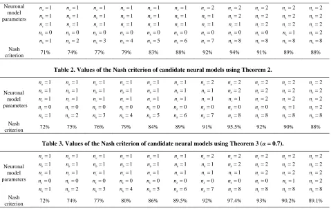
The flowchart of this algorithm is given in Figure 2. 2.4. Validation Tests of the Neuronal Model The neuronal model obtained from the estimation of its parameters is valid strictly used for the experiment. So check it is compatible with other forms of input in order to properly represent the system operation to identify. Most static tests of model validation are based on the criterion of Nash, on the auto-correlation of residuals, based on cross-correlation between residues and other inputs to the system. According to [49], the Nash crite-rion is given by the following equation:
21
2
1 1
ˆ
( ) ( )
100% 1
1
( ) ( )
N
k
N N
k k
y k y k
Q
y k y k
N
(72)
N is the number of samples.
In [50-52], the correlation functions are: - autocorrelation function of residuals:
1 1 1
2
1 1
( )
1 1
( ) ( ) ( ) ( )
1
( ) ( )
ee
N N N
k k k
N N
k k
R
e k e k e k e k
N N
e k e k
N
(73) - crosscorrelation function between the residuals and the previous entries:
1 1 1
2 2
1 1 1 1
( )
1 1
ue
N N N
R
( ) ( ) ( ) ( )
1 1
( ) ( ) ( ) ( )
k k k
N N N N
k k k k
u k u k e k e k
N N
u k u k e k e k
N N
(74) Ideally, if the model is validated, the results of correla-tion tests and the Nash criterion following results:
( ) 1, 0
0, 0
ee
R
, Rue( ) 0 and Q100%.
Typically, we verify that and the func-tions
100%
Q
1.96 1.96
R
N N
.
3. Adaptive Control of Complex Dynamic
Systems
In this section, we propose a structure of neural adaptive control of a complex dynamic system and three learning algorithms of a neuronal controller.
3.1. Structure of the Proposed Adaptive Control In this work, the architecture of the proposed adaptive control is given in Figure 3.
The considered neural network is first trained off-line to learn the inverse dynamics of the considered system from the input-output data. The model following adap- tive control approach is performed after the training pro- cess is achieved. The proposed Lyapunov-Base training algorithm is used to adjust the considered neural network weights so that the neural model output follows the de- sired one.
3.2. Learning Algorithms of Neural Controller Three learning algorithms of the neural controller are proposed.
Theorem 4. Learning the neuronal controller may be effected by the following equation:
1
2 2
1
1 1
1
1
ˆ 1
1 wc k
wc k
y k u k
1 1
ˆ c
wc k wc k
y k e k
wc k
(75)
with:
1, 1, 1, 1 0
(76)
1
1
1
1
1
1
1
1
1
(77)
r is the reference signal.
ˆc
e k r k y k
r k y k
(78)
a
y kn
On-line update of
ANN by +
-
System
Recurrent Neural Network Reference
1
y k
y k
1
z
1
z
1
z
1
z
1
u k
r k
m r k
c
r kn
2
u k
b
u kn
[image:9.595.312.535.83.288.2]
Figure 3. Structure of the proposed adaptive control.
1 1 2 2
11 11 1
3 3 4 5
11 1 11 11
5 6 6 7
1 11 11
, , , , , ,
, , , , ,
, , , , ,
h r h
h
r h h
n n n
n
T
n n n
wc wc wc wc wc
wc wc wc wc
wc wc wc wc
are the weight of the neuronal controller. Proof:
The control system consists of using an optimization digital non-linear algorithm to minimize the following criterion:
21
2 2 2
1 2
2 2 2
1 1 1
c c c
J k e k e k wc k
u k
(79)
with:
1
ˆ 1 , ,ˆ , 2 , , ,
, , , ,
r
a b
T T
c n
k y k y k n u k u k n
r k r k n k k
(80)
7
3
11 1
1
1 2
h
n
h j j j
u k wc u k wc xc k
5 4
1 11
1
r
n i i i
wc k wc
(81)
1
, , h
T
h h h
n
xc k xc k xc k (82)
1
h
j j
xc k f sc k (83)
1
, , h
T
c n
1
6
1 1 2 1 1 hj jm m jm m
m m
j
sc k wc k wc xc k
wc
nr
nh(85)
1
1
u k u k u k
2
(86)
1
c c c
e k e k e k
(87)
The minimum of criterion Jc
k
is reached when:
0c
J k
wc k
(88)
The solution of Equation(88) calculates the weight of the neuronal controller as follows:
1 1 1 1 1 1 1 1 1 c c c c e kwc k wc k e k
wc k
e k u k
e k u k
wc k wc k
(89)
The term e kc
defined by:
1 1 1 1 1 1 2 2 1 1 1 1 1 1 1 1 T c c T c c c c c c c c c e ke k wc k
wc k
e k e k
e k
wc k wc k
e k e k wc k u k u k wc k
e k e k
e k e k
wc k wc k
u
2 2 1 1 1 1 2 1 1 2 2 1 1 1 1 1 1 1 1 1 T c c c c c T c c c c ce k u k
k
wc k wc k
e k e k
e k e k
wc k wc k
e k u k
u k
u k wc k
e k e k
e k e k
wc k wc k
2 1 1 1 c u k e k wc k (90) therefore:
2 1 1 c c c e k e k wc k e k 2 2
1 1
1 1
1
1 e kc u k
wc k wc k
(91)
Using the above equations, the relationship giving the vector wc k
1
minimizing the criterion Jc
k canbe written as follows:
2 1 1 2 2 1 1 1 1 2 1 1 1 2 2 1 1 1 1 1 1 1 1 1 1 1 1 c c c c c c c c c wc e k wc k wc k e k e k wc ke k u k
wc k wc k
u k e k
wc k e k
wc k
e k u k
wc k wc k
e k
wc k e k
w 1 1 1 1 1 c k
k e
c e k wc k
2 1 1 2 2 1 1 1 1 2 1 1 2 2 1 1 1 1 1 1 2 2 1 1 1 1 1 1 1 1 1 1 1 1 1 c c c c c c c k e k wc ke k u k
wc k wc k
u k wc k
e k u k
wc k wc k
e k
wc k e k
wc k
e k u k
wc k wc k