The Analysis of Real Data Using a Stochastic Dynamical
System Able to Model Spiky Prices
*#
Lorella Fatone1, Francesca Mariani2, Maria Cristina Recchioni3, Francesco Zirilli4 1Dipartimento di Matematica e Informatica, Università di Camerino, Camerino, Italy
2CERI—Centro di Ricerca “Previsione, Prevenzione e Controllo dei Rischi Geologici”,
Università di Roma “La Sapienza”, Roma, Italy
3Dipartimento di Scienze Sociali “D. Serrani”, Università Politecnica delle Marche, Ancona, Italy 4Dipartimento di Matematica “G. Castelnuovo”, Università di Roma “La Sapienza”, Roma, Italy
Email: [email protected], [email protected], [email protected], [email protected]
Received October 28,2011; revised November 25, 2011; accepted December 15, 2011
ABSTRACT
In this paper we use filtering and maximum likelihood methods to solve a calibration problem for a stochastic dynami- cal system used to model spiky asset prices. The data used in the calibration problem are the observations at discrete times of the asset price. The model considered has been introduced by V. A. Kholodnyi in [1,2] and describes spiky asset prices as the product of two independent stochastic processes: the spike process and the process that represents the asset prices in absence of spikes. A Markov chain is used to regulate the transitions between presence and absence of spikes. As suggested in [3] in a different context the calibration problem for this model is translated in a maximum like- lihood problem with the likelihood function defined through the solution of a filtering problem. The estimated values of the model parameters are the coordinates of a constrained maximizer of the likelihood function. Furthermore, given the calibrated model, we develop a sort of tracking procedure able to forecast forward asset prices. Numerical examples using synthetic and real data of the solution of the calibration problem and of the performance of the tracking procedure are presented. The real data studied are electric power price data taken from the UK electricity market in the years 2004-2009. After calibrating the model using the spot prices, the forward prices forecasted with the tracking procedure and the observed forward prices are compared. This comparison can be seen as a way to validate the model, the formu- lation and the solution of the calibration problem and the forecasting procedure. The result of the comparison is satis- factory. In the website: http://www.econ.univpm.it/recchioni/finance/w10 some auxiliary material including animations that helps the understanding of this paper is shown. A more general reference to the work of the authors and of their coauthors in mathematical finance is the website: http://www.econ.univpm.it/recchioni/finance.
Keywords: Stochastic Dynamical System; Inverse Problem; Spiky Prices; Data Time Series Analysis
1. Introduction
A spike in an asset price is an abrupt movement of the price followed by an abrupt movement of approximately the same magnitude in the opposite direction. The modeling of spikes in asset prices is a key problem in finance. In fact spiky prices are encountered in several contexts such as, for example, in electric power prices and, more in general, in commodity prices.
In this paper the model introduced by V. A. Kholodnyi in [1,2] to describe spiky prices is combined with some
ideas introduced by the authors and some coauthors to study calibration problems in mathematical finance, see [3-9]. That is we introduce a stochastic dynamical system to model spikes in asset prices and we study a calibration problem for the dynamical system introduced. The method proposed to solve the calibration problem is tested doing the analysis of data time series. We consider synthetic and real data. The real data studied are electric power price data taken from the UK electricity market in the years 2004-2009.
Following V. A. Kholodnyi (see [1,2]) we model spiky asset prices as a stochastic process that can be represented as the product of two independent stochastic processes: the spike process and the process that describes the asset prices in absence of spikes. The spike process models spikes in asset prices and it is either equal to the multiplicative amplitude of the spike during the spike
*The research reported in this paper is partially supported by MUR— Ministero Università e Ricerca (Roma, Italy), 40%, 2007, under grant: “The impact of population ageing on financial markets, intermediaries and financial stability”. The support and sponsorship of MUR are grate-fully acknowledged.
periods or equal to one during the regular periods, that is during the periods between spikes. The second stochastic process of the Kholodnyi model describes prices in ab- sence of spikes. This last process has been chosen as a diffusion process. Finally we use a two-state Markov chain in continuous time to determine whether asset prices are in the spike state, that is during a spike, or in the regular state, that is between spikes.
The model for spiky asset prices studied depends on five real parameters. Two of them come from the process that describes the asset prices in absence of spikes, one of them comes from the spike process and the last two parameters come from the two-state Markov chain used to model the transitions between spike and regular states.
The calibration problem studied consists in estimating these five parameters from the knowledge at discrete times of the asset prices (observations of the spiky prices). That is the calibration problem is a parameter identification problem or, more in general, is an inverse problem for the stochastic dynamical system that models the asset prices. This calibration problem is translated in a constrained optimization problem for a likelihood function (maximum likelihood problem) with the likelihood function defined through the solution of a filtering problem. The likelihood function is defined using the probability density function associated with the diffusion process modeling asset prices in absence of spikes. This formulation of the calibration problem is inspired to the one introduced in [3] in the study of the Heston stochastic volatility model that has been later extended to the study of several other calibration problems in mathematical finance (see [4,5,8, 9]).
The filtering and the maximum likelihood problems mentioned above are solved numerically. The resulting numerical solution of the calibration problem determines the values of the (unknown) parameters that make most likely the observations actually made. Note that in the processing of numerical data to improve the robustness and the quality of the solution of the calibration problem some preliminary steps are introduced in the optimization procedure used to solve the calibration problem and the results obtained in these preliminary steps are used to penalize the likelihood function obtained from the filtering problem. That is the maximum likelihood problem originally formulated in analogy to [3] is reformulated adding penalization terms to the likelihood function and choosing an ad hoc initial guess for the optimization procedure to improve the robustness and the quality of its solution. This reformulated optimization problem is solved numerically using a method based on a variable metric steepest ascent method.
Furthermore, as a byproduct of the solution of the filtering problem, we develop a tracking procedure that, given the calibrated model, is able to forecast forward
asset prices.
The method used to solve the calibration problem and the tracking procedure are used to analyze data time series. Numerical examples of the solution of the calibration problem and of the performance of the tracking pro- cedure using synthetic and real data are presented. The synthetic data are obtained computing one trajectory of the stochastic dynamical system that models spiky asset prices. We generate daily synthetic data for a period of two years. The first year of data is generated with one choice of the model parameters, the second year of data is generated with a different choice of the model para- meters. The second year of data is generated using as initial point of the trajectory the last point of the first year of data. In the solution of the calibration problem we choose as observation period a period of one year, that is we use as data the daily observations corresponding to a time period of one year, and we move one day at the time this observation period through the two years of data. The calibration problem is solved for each choice of the observation period. The two choices of the model para- meters used to generate the data and the time when the model parameters change value are reconstructed satis- factorily by the calibration procedure. The real data studied are daily electric power price data taken from the UK. electricity market. These electric power price data are spiky data. We choose the data of the calibration problems considered as done above in the study of synthetic data extracting the observation periods from a time series of five years (i.e. the years 2004-2009) of daily electric
power (spot) price data taken from the UK market. The results obtained show that the model is able to establish a stable relationship between the data time series and the estimated model parameter values. Note that in the real data time series for each observation day we have the electric power spot price and the associated forward prices observed that day for a variety of delivery periods. That is for each spot price there is a set of forward prices associated to it corresponding to different delivery periods. Moreover in the calibration problem only spot prices are used as data. To exploit this fact we proceed as follows. After calibrating the model using as data the spot prices observed in the first three years of the data time series, we use the calibrated model, the tracking procedure and the spot prices not used in the calibration to forecast the forward prices associated to these last spot prices. We compare the forward prices forecasted with the tracking procedure with the observed forward prices. The comparison is satisfactory and establishes the effectiveness of the model, the validity of the proposed formulation and solution of the calibration problem and the quality of the forecasted prices.
is able to capture only one property of the electric power prices: the presence of spikes. It does not consider, for example, the mean-reverting property and the presence of weekly and season cycles in electricity prices. This study aims to be a first attempt to solve, with the strategy presented in Section 3, calibration problems involving stochastic dynamical systems that can be used to describe electric power prices. That is the methodology discussed in this paper can be applied in the calibration of more sophisticated stochastic dynamical models that can be used in electricity markets (see for example [10]).
The website: http://www.econ.univpm.it/recchioni/fi- nance/w10 contains some auxiliary material including some animations that helps the understanding of this paper. A general reference to the work of the authors and of their coauthors in mathematical finance is the website:
http://www.econ.univpm.it/recchioni/finance.
The paper is organized as follows. In Section 2 we describe the model for spiky asset prices. In Section 3 we formulate and we solve the filtering and the calibration problems for the model presented in Section 2 and we introduce the tracking procedure used to forecast forward prices. In Section 4 some numerical examples of the solution of the calibration problem and of the performance of the tracking procedure introduced in Section 3 using synthetic and real data are presented.
2. The Stochastic Dynamical System for
Spiky Asset Prices
Let us introduce a stochastic dynamical system used to model spiky asset prices, see [1,2]. In this model the spiky prices are defined as the product of two stochastic processes: the spike process and the process that describes asset prices in absence of spikes. As said in the Intro- duction the transitions between spike and regular states are regulated through a two state Markov chain in continuous time.
Let t be a real variable that denotes time, Mt, t
(continuous time) two-state (i.e. regular state, spike
state) Markov chain and let
0, be the
,
,
, ,, ,
ss sr
rs rr
P T t P T t
P T t t T
P T t P T t
0 < ,
denot
e rly de e t on
te that the Chapman-Kolmogorov equation for the M
(1)
be its transition probability matrix. Note that in (1)
ss nd Prs e the transition probabilities
of going from the spike state at time t respectively to th
spike or to the regular state at time T, and simila
,sr
P T t and Prr note th probabilities
of going from the regular state at time t respectively to the
spike to the regular state at time T.
No
2 2
,t a
or
P T
T t,
T t, ransitiarkov chain Mt, t0, can be written as follows:
, =
, ,P T t P t
( ,
for every , , such that 0 < ,
T P
t T t T
2)
together with the condition that P T t
, is the 2 2 identity matrix when t= .TLet 0 <tT and p tr
, p ts
, p Tr
, p Ts
regular
be resp he pro in e
state and in the spike state at time t and at time T.
We have:
ectively t babilities of be g in th
=
,
, 0 <s s
r r
p T p t
P T t t T p T p t
. (3)
In the time-homogeneous case it is possible to write an ex
plicit formula for the matrix P T t
, , tT, as a func-tion of the parameters that define the g eratoren of
,P T t , tT. These parameters control the duration
an cy of the spikes, that is they control the expected lifetime of the spike periods and the expected lifetime of the periods between spikes. It is easy to see that in the case of a time-homogeneous Markov chain
t
d the frequen
M , t0, the transition probability matrix P T t
, , t0 < T, is a function only of the difference Tt,
and that we have [1]:
( )( )
e T t
b a
( )( )
( )( ) ( )( )
e
, = , 0 < ,
e e
a b T t a b
T t a b T t a b
b b a b a b
P T t t T
a a a b a b a b
(4) where anda are non negative real parameters. M
a
b
th
ore- over we ssume at a b, are not both zero.
From now on in o odel for spiky prices we always as
ur m
sume that the two-state Markov chain Mt, t0, is
time-homogeneous and, as a consequence me that its transition probability matrix P T t
, , 0 <t T,, we assu
is given by (4).
The process that describes the asset prices in a of
bsence
(5)
with the initial condition:
(6) where denotes the rando
spikes is a diffusion process defined through the fol- lowing stochastic differential equation:
ˆ ˆ ˆ
d =St S ttd S Wtd t, t>0,
* 0 =Sˆ ,
ˆ
S
ˆ > 0t
S
et pric
m variable that describes the ass e in absence of spikes at time t, > 0,t
,
are constants, Wt, > 0,t is the standard W
0= 0,
W dWt, t tochastic differen-
tial and the rand a is a given initial condition. For simplicity we assume th the random variable Sˆ* is concentrated in a point with probability one and, with abuse of notation, we denote this point
*
ˆ
iener pr
with ocess,
S . Recall
> 0, is ble Sˆ* its s
at om
that
vari > 0
> 0
is the volatility coefficient.
Equation (5) def s the asset price namics of the celebrated Black les model. Note that the soluti
ine dy
-Scho on of
(5), (6) is a Markov process known as geometric Brownian motion. Note that several other Markov processes different from the one defined in (5), (6) can be used to model asset price dynamics in absence of spikes. For example we can use one of the so called stochastic volatility models that have been introduced recently in mathematical finance to refine the Black-Scholes asset dynamics model.
Let us define the spike process t, t0, that models
the amplitude of the spikes in the asset prices. Let t,
ity
0, be a stochastic process d independent positive random variables with given probability dens
ns
t, ,t
functio
ma e of
> 0, t0. We assume that if the
Markov chain Mt, t0, is in the regular state then
the spike process t, t0, is equal to one. If the
Markov chain Mt, t0, transits from the regular state
to the spike state at time , > 0, then the spike pro- cess t, t0, a value sampled from the
random variable
is equal to
during the ent e period begin- ning with =
ire tim
t that the Markov chain Mt, t0,
remains in the spike state. We assume that Mt, t0,
is in the regular state me t= 0 with probability
the spike process t
at ti one,
so that starts with 0= 1 with one. Let us observe that in the case of sp s with constant amplitude > 1,
e
pro-bability ik
the probability ensity func-
t, =
,d
tion > 0, t0, is the Dirac delta
function
with support in = , we have:
t, =
, > 0, t (7)
that is
0.
lly we say that the spike process
Fina t, t0, is in
hain the spike state or in the regular state if the Markov c
, t
M t0, is in the spike state or in state
respectively. In our model for spiky prices we assume kes have constant amplitude > 1,
the regular
that the spi that is
we assume (7).
Let us define now the process that de s the asset prices with
scribe
spikes. Let us denote with St > 0 the
at the s random variable that models the price (eventually) with spikes of the asset at time t0. We assume th pike
process t, t0, and the process Sˆ ,t t0, that
describes asset prices in abs of spikes, are independent. Followin ,2 efine the process St t s the
product of the spike process t,
ence
g [1 ] we d , 0, a t0, and of the process Sˆ ,t t0, that is:
ˆ
= ,
t t t
S S t0. (8)
te that the process pike state or in No
is in the s the
, t
S
the
0,
t
regular
, t
for spiky asset prices state depending from fact that the spike process t0, is in the spike
state or in the regular state respectively, or equivalently,
depending from the fact that the M kov car hain Mt, 0,
t is in the spike state or in the regular state
respectively.
1] it has been shown that the process St, t> 0,
is able to rep In [
se
depend
roduce spikes in asset prices. This can be
, t
S
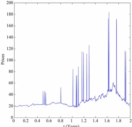
that en in Figure 1 where synthetic data sampled f
> 0,
t are shown. These synthetic data are those used in
the numerical examples presented in Section 4. Note ing on the values of the parameters defining the model, the trajectories of St, t0, can exhibit a
variety of behaviours. In particular, when t,
rom
M t0, is
time-homogeneous and a0, b0, the expected times
s
t and tr spent by the process St, t> 0 i ike
mode” and in “regular ( ke) mode”, respec- vely, ar given by (see [1]):
, n “sp
i.e. inter-spi
ti e
1 1
= , =
s r
t t
a b. (9)
If
s
t is small in comparison w
time of change of the process the pr ss
condition ca
ith the characteristic
ˆ ,t
S
ne
> 0,
t
n (5 then oce St, t> 0, exhibits spikes. For example, if Sˆ ,t > 0,
t is the diffusion process defi d i ) then the
previous n be stated as follows:
2
2 = 1 and = 1.
s s
t t
a a
(10)
We interpret ts as the expected lifetim
and
e of a spike,
r
t as the expected time elapsed bet two
co e
l
ween
e nsecutive spik s. That is the parameters a and b
contro the duration and the frequency of the spikes through (9). For example, the relations (9) sugg st that in order to model short-lived spikes the parameter a must
[image:4.595.308.536.493.713.2]be large, while to model rare spikes the parameter b must
be small.
Using some heuristic rules to recognize spikes on the data time series considered thank to their relation with the spike duration and frequency a rough estimate of the parameters and can be obtained directly from observed s pri arket data). For example, the relations ge at initial estimates and of
and obtained as follows:
a
piky (9) sug
resp
b
ces (m st th
ectively, can be
0
a b0
a b
0 0
0 0
1 1
= , =
s r
a b
t t , (11)
where 0
s
t and tr0
rom
are computed (using some heuristic rules) directly f the data available as the observed average lifetime of the spikes and the observed average time between two consecutive spikes, respectively.
Finally it is easy to see that the asymptotic probabilities of the time-homogeneous Markov chain Mt,
regular stat 0,
t of being in the spike and in the es ar
respectively:
e
=π = ,
=π = .s s pr r
a b a b
(12)
With the previous choices the model for spiky asset prices introduced in 1,2] depends on five parameters, that is: , , , , .a b
b a
[
p
The parameters and are those appearing in (5) and are relative to the asset rice model in absence of spikes, the remaining parameters are
e to the spike process (i.e.
p
relativ ) and to the Markov chain th
gular
at regulates the transitions states (i.e. a b, ).
between spike and re-
3. The Filtering and the Calibration
Problems
The parameters , , a, b, are grouped in the
following vector:
= , , , , ,T a b
(13)
where the superscript denotes the transpose operator. The vector
T
is th nown of the calibration pro- blem that must be d ined from the data a
The vectors
e unk
eterm vailable. , descri g admissible sets of parameter va
bin
lues, must satisfy some constraints, that is we must have where:
5
= = , , , , T 0, 0, 0, 1 ,
a b a b
(14) and 5 is the five dimensional real Euclidean space.
The constraints contained in express some ele- mentary properties of the mode oduced in Section 2.
l circum-
ration problem are the observation
where
l intr
Note that, when necessary to take care of specia stances, more constraints can be added to .
The data of the calib
times: 0 =t0<t1 t2 t and the spiky asset price Si observed
< << n< ,
at time ti,
* 0 = ˆ0 = ˆ .
S S S The observed price Si
ber that is understood as being
i
to
= 0,1, , ,
i n
is a positiv
num
e real sampled from the random variable Sti, = 0,1, , . n Starting from these
data we want solve the following problems:
Calibration Problem: Find an estimate of the vector
= , , , T a b,
.
Filtering Problem (Forecasting Problem): Given the
value of e vector th =
, , , ,
T a b
estimated fore- cast the forward asset prices.
Note that the prices Sj,
wi
= 0,1, , ,
j n
th forward asset prices future”, that is, in our
are called spot asset prices and that we mean prices “in the setti
ot pr
ferent delivery pe
used in real markets, in fac
s o s a available and parison betw
der ome of) the
009 and w
Let us mention t he forecasted forward asset prices as
ikes (see [1,2] for more de
ng, we mean the forward prices at time ti associated to the sp
ice Si, i= .n These are the prices at time ti of the
asset with delivery time t> ,ti i= .n Let us point out
that in correspondence of a spot price we can forecast several forward prices associated to dif
riods. The delivery periods of interest are those actually t for these delivery period bserved forward price re a com- een observed forward prices and forecasted forward prices is possible. In Section 4 in the analysis of real data we consi (s delivery periods used in the UK electricity market in the years 2004-2
e make this comparison. hat t
sociated to the spiky price model introduced in Section 2 do not exhibit spikes while, of course, the corresponding (spot) asset prices exhibit sp
tails).
The calibration problem consists in estimating the value of the vector that makes “most likely” the observations. The observations available at time t> 0
are den tedo with:
= : , > 0.
t Si tit t
(15) Note that for simplicity we assume that the transitions from regular state to spike state or viceversa happen at the observation times.
Let p S t
ˆ, t,
, ˆ > 0,S > 0,t be the probabilitydensity function of the stochastic process ˆSt at time
> 0
t conditioned to the observations t and let
ˆ,
= ˆ, ,
,i ti
p S t p S t ˆ > 0,S ti<tti1, be the probability density function of the stochastic process Sˆt
conditioned to the observations made up to time =t ti,
when ti<tti1, = 0,1, , ,i n where for convenience we define tn1=.
The probability density functions i
ˆ,
, 1<
i t ti
ˆ
S0,
p S t
t , , = 0,1, , ,i n are the solutions of
equation associated to the Black-Scholes model (5): for = 0,1, , ,i n
2 2 2
2
1
ˆ 0, i < i , ,
S S
S t tt
1 ˆ ˆ
= ˆ ˆ,
2
i i i
p p p
S S
t
(16)
ˆ,
=
i i
p S t f Si ˆ; , Sˆ0, , (17)
where
*
0 ˆ; = ˆ ˆ , ˆ> 0, ,
f S SS S (18)
ˆ; = ( )
ˆ
ˆ ,ˆ , 2 ,
i r i i s i
f S p t S S p t S
S
> 0, = 1 , , ,
i S i n 9 and (1 )
where pr
ti s
ilities defined through the time-homogeneous
t
p t are, respectively, the proba-
bi Markov
chain M , t0, of being in the regular a
the initial value problem
be written as follows: nd in the spike state at time t= ,ti i= 0,1, , n (see (3)).
The probability density functions pi, i= 0,1, , , n
solutions of s for the Fokker- Planck Equations (16)-(19), can
0
1
ˆ, = dˆ ˆ, , ,ˆ ˆ;
ˆ 0, < , = 0,1, , , ,
i f i i
i i
p S t S p S t S t f S S t t t i n
, where (20) f p qis the fundamental solution of the Fokker- Planck E uation (16) associated to the Black-Scholes model (5), that is:
2 2 2 ˆ 1 log ˆ 2 2 1ˆ, , ,ˆ =
ˆ 2π
e ,
ˆ 0, ˆ 0, , 0, > 0.
S S t t tt
In o ure the likelihood of the vector
f
S
t t S
t t
p S t S t
S t t
(21)
rder to meas we
introduce the following (log-)likelihood function:
1
1 1
=0
=n log i i ,i , .
i
F p S t
(22)It is worthwhile to note that definition (22) contains an important simplification. In fact a more correct d
of the (log-)likelihood function should be:
efinition
1
1 1
=0
=n log i i ,i , ,
i
F p S t
(23)
where Si1=Si1 or
1 1= i
i S S
depending on whether
at time the asset price is in the regular state or in the
spike state respectively, However, since when dealing with real decision about the character of the ke state) of the observed prices is dubi o adopt the de- finition (22) for the tion. In fact the choice made in (22), at oducing some inaccuracy, avoids the ng a (du criterion to recognize re order to evaluate the (log-)likelihood function. The validity of
th e
intro- duced in (22) using
1
i
t
= 0,1, , 1.
i n
financial data the state (regular or spi
ous, we prefer t (log-)likelihood func
the price of intr necessity of defini
gular and spike states in
1
bious)
is choice is supported by the fact that in the num rical experience shown in Section 4 the simplification
i
S instead of Si1,
= 0,1, , 1,
i n
results.
n s
is sufficient to obtai atisfactory
The solution of the calibration problem is given by the vector that solves the following optimization pro- blem:
. maxF
Problem (24) is aximum d problem. the vector
(24)
called m likelihoo In fact *
n
alg
tion of (24) is the vector
that ma made.
solu kes “most likely” the
(2
ear inequal
e the maxi- mum likelihood p
steepest ascent method. T riable metric te
observations actually
ity c
to s
he va
Problem 4) is an optimization problem with nonlinear objective function and li onstraints.
Note that (22), (24) is one possible way of formulating the calibration problem considered using the maximum likelihood method. Many other formulations of the calibration problem are possible and legitimate. Moreover the formulation of the calibration problem (22), (24) can be easily extended to handle situations where we con- sider calibration problems associated to data set different from the one considered here, such as, for example, data set containing asset and option prices or only option prices.
The optimization orithm used olv
roblem (22), (24) is based on a variable metric
chnique is used to handle the constraints.
Let be the absolute value of , and be the Euclidean norm vector ning from an initial guess:
of the . Begin
0
T0= 0, , , , 0 0 0 ,
a b
(25)
we update at every iteration the current approximation of the solution of the optimization problem (24) with a step in the direction of the gradient with respect to com- puted in a suitable variable metric of the (log-)likelihood function (22).
In particular let us fix a tolerance value tol> 0 and a maximum number of iterations iter> 0. Given
0
=
the optimization procedure can be sum-
2) Evaluate
k .F If > 0k and
1< ,
k k
F F tol go to item 7;
3) Evaluate the gradient of the (log-)likelihood func- tion in = k, that is:
= , , , ,
.T
k F F F F F k
F
a b
(26)
If
k <F tol
go to item 7;
4) Perform the steepest ascent step, evaluating
1
= ,
k k k
k F
where k
T
is a quantity that is used to define the the step made. he quantity k can
be chosen as a scalar or, more in general, as a m trix of a suitable dimensions. The choice of k involves the use
of the “variable metric”. When k is chosen to be a
scalar we have a “classical” steepest ascent method; 5) If k 1 k < ,
tol
go to item 7;
6) Set k=k1, if k<iter go to item 2;
7) Set *=k
and stop.
The vector * obtained in step the (nume proximation of the maximizer of the (log-) likelihood function.
7 is rically computed) ap
show the (log-) likelihood function
Numerical experiments have n that
F defined in (22) is a flat func-
tion. That is there are many different ctve ors in that make likely the data. ization of obj fu
epest as to solve the
corresponding optimization problems (i.e.: (24)), special
atten- tion must be paid to the choice of the init
of the optimization procedure. That is in actual computations a “good” initial gue
ective In the optim
nctions with flat regions when local methods, such as the ste cent method, are used
ial guess
ss 0
iis mportant to “g
sp ro m
find a More ood” solution of the optimization problem (24). ecifically in the p ble considered here the use of good initial guesses of the volatility and of the drift improves substantially the quality of the estimates of all the parameters contained in the vector . That is in the solution of problem (24) the parameters and are the most “sensitive” parameters of the vector .
hese d e e robustne For t reasons in or er to improv h
th on of pro (24) that is obtained with the
op ion meth is seful to
in a
t ss of e soluti blem
d above it u timizat od describe
troduce some d hoc steps that lead to a simple refor- mulation of the (log-)likelihood function (22), of the calibration problem (24) and of the method used to solve problem (24). First of all an ad hoc preliminary simplified optimization problem is solved to produce a high quality initial guess for the steepest ascent method summarized in steps 1) - 7). We proceed as follows. First we estimate two initial values of and , let us say and , directly from the data available, that is we com- pute the historical volatility and the historical drift of the data available (see, for example, [11]). These
estimates are used as initial guesses to maximize the objective function (22) as a two variables function of the parameters and , with the constraint > 0. Note that in this preliminary step we consider as data used to define the (log-)likelihood function (22) only the “most regular portion of the input da ”. The most regul portion of the input data is chosen using elementary empirical rules that try to find one or mo regular periods in the data considered. In this preliminar optimi ation problem the remaining components of the vec r
ta ar
re
y z
to are initialized as follows = = 0= 0= 0
a b a b and
0
= = 1
and these initial values are kept constants in the optimization procedure with respect to and . Let
*, *
be the maximizer found at the end of this preliminary step. In order to keep memory in the maximum likelihood problem (24) of the values * and*
found in the preliminary step we add to the objective function (22) the following penalization term:
2 2
* *
1 2 , > 0,1 2> 0,
k k k k (27)
where k1, k2 are positive penalizat n const s. That is we conside e following modified (log-)likelihood func- tion:
io ant r th
2 2
* *
1 2
1
1 1 =0
2 2
* *
1 2
1 2
=
= og ,
,
> 0, > 0, .
n
i i i
i
F F k k
p S t
k k
k k
l
(28)
The variable metric steepest ascent method 1) - 7) is now applied to solve problem (24) when the (five varia- bles) (log-)likelihood function F defined in (28) re laces
the (log-)likelihood function
p
F defined in (22) sta
from the in
rting itial guess:
0= *, *, , ,0 0 0 T ,
a b
(29)
where the initial values 0
a and b0 are estimate irec-
from the input data through (11) and, finally, the ini- tial value 0
d d tly
is chosen as a rough estimate of the ave- rage am of the s appearing in the input data. That is prob (24) is so ed rep
plitude lem
pikes
lv lacing F with F start-
ing from n itial guess that uses the results obtained in the preliminary step of the optimization procedure and tries to exploit the data using the “physical” meaning of the model parameters.
a in
These ad hoc steps used to reformulate problem when applied to the analysis of synthetic data, lead t substantial improvement in the accuracy of the estim of the model parameters obtained when compared to estimates obtained solving directly (22), (24) and to a great saving in the computational cost of solving the ca- (24),
libration problem. This reformulation of problem (24) is used to analyze the data considered in Section 4.
As a byproduct of the solution of the calibration pro- blem we obtain a technique to forecast forward prices. Let us consider a filtering problem. We assume that the vector
asset
to the data
solution of the calibration problem associated t =
Si:tit
, t=tn> 0 isknown. From the knowledge of =
, , , , a b
T attime t=tn we can forecast the forward asset prices with
delivery period t> 0 deep in the future and delivery
time n=tn t as follows:
t ,
=
i n i
S
ˆ
ˆ = 1
, i
r i s i
S
p p S
e i ti, ti
=i ti t i= ,n
(30) where
denotes the expected value of
.In the numerical experiments presented in Section 4 we use the following approximation:
9 =01
ˆ , = .
10
ti i k
k
S
S i n (31)
Note that using formula (31) we have implicitly assumed
> 9
n . In fact in the data time series considered in Sec-
tion 4 the average in time of the (spiky) observations appearing in (31) gives a better approximation of the “spatial” average
ˆti
S
of the price without spikes than the individual observation Si made at time t=ti of the
spiky price. However the average in time of the obser- vations approximates the “spatial” average only if short tim
s
) an average of piky price ted value of non spi .
The first numerical experiment presented consists in solving the calibration problem discussed in Section 3 using synthetic data. This experiment does the analysis a time series of daily data of the spiky asset price duri a period of two years. The time series studied is made of 730 daily data of the spiky asset prices, that is the p
time a ave been
ectory at time e periods are used. This is the reason why we limit the mean contained in (31) to the data corresponding to ten consecutive observation times, that is corresponding to a period of ten day when we process daily data as done in Section 4. Note that in (31 s s is used to approximate the expec ky prices
4. Numerical Results
of ng
rices
i
S at ti, i= 0,1, ,729. These dat h
obtained computing one trajectory of the stochastic dy- namical system used to model spiky asset prices defined in Section 2 looking at the computed traj
= i
t t , i= 0,1, ,729, with ti ti1= 1 365,
chosen and
where we have
=
i 1, 2, , 729, t0= 0
*
0 =Sˆ0 =Sˆ = 20. We choose the vector
S that spe-
the model used to generate the data equal to cifies
1
= , , , , T = = 0.03, 0.3, 70, 1, 2T a b
in the
first year of data (i.e. when t=ti, i= 0, 1, , 364), and
equal to =
, =
2= 0.1,
0.8, 150, 5, 4
T T
in the second year of data (i . when t= ,ti = 365, 366, , 729
i ). The data are generated using as
initial value of the second year the last datum of the first year. The synthetic data generated in this way are shown in Figure 1. These data are spiky data and the fact that the first year of data is generated using a different choice of
, , ,a b .e
than the choice made in the second year of data can be seen simply looking at Figure 1.
We solve problem (24) with the ad hoc procedure described in Section 3 using the data associated to a time window made of 365 consecutive es, that
we m ss
ding t ding
observation tim ove this window acro he datum correspon is 365 days (one year), and
the two years of data discar
to the first observation time of the window and inserting the datum corresponding to the next observation time after the window. Note that numerical experiments sug- gest that it is necessary to take a large window of obser- vations to obtain a good estimate the parameters a, b
and . The calibration problem is solved for each choice of the data time window applying the procedure described in Section 3, that is it is solved 365 times. The 365 vectors constructed in this way are compared to the two choices of the model parameters used to
ta. Moreover the time w
generate the da hen changes from being 1 to being 2 is reconstructe
To represent the 365 vectors obtained solving t ata time windows considered, we a ate ucted vector
d.
he ca- problem in correspondence 365 d
ssoci t reconstr
libration to the
o each
5 R
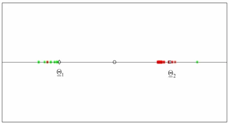
.
Let us explain how this correspond vectors
a point on a straight Figure 2) ce is established. We rst represent the
line (see en
[image:8.595.309.538.577.700.2]fi 1 and 2 that generate the data as two points on the straight line mentioned above having a distance proportional to 1 2 * measured in 1* units, where
Figure 2. Reconstruction of the parameter vectors 1 and .
2
* 5
=1 1 =
5 i i
and
5= 1 , 2 , , 5 T R
. We choose the origin of the straight line to be the mid point of the segment that joins 1 and 2. In Figure 2 the diamond epresents the vector
r 1
and the square represents the ctor ve 2. The unit length is 1*. The vectors (points) solution of the 365 calibration problems are represented as (green or red) stars. A point P= is plotted around 1 when
the quantity
* 1 * 1
is smaller than the quantity
* 2 * 2
, otherwise the point P is plotted around 2.
The distance of the point P from 1 is plotted
ro
P
when und
a 1 (or from 2 when P is plotted around ) is 1 * measured in 1* units (or 2
* 2
measured in 1* units). The point P=
plotted around 1 is plotted to the right or to the left of 1
according to the sign of the second component of 1
(negative second component of 1 is
plotted to the left of 1). Remind that the second com- ponent of is the volatility coefficient . A similar statement holds for the points plotted around 2. The results obtained in this experiment are show Figure 2. In this figure the green stars represent the solutions of the calibration problems associated to the first data tim
while the red stars represen
second “half” of the data time windows is the second 182 time win shows that the points (vectors) obtained solving the calibration
n in
183
t those associated to the (that
e windows, that is the first “half” of data time windows,
dows). Figure 2
problems are concentrated on two disjoint segments one to the left and one to the right of the origin and that they form two disjoint clusters around 1 and 2. That is, the solution of th 365 calibration problems corresponding to the 365 time windo scribed previously shows that two sets of parameters seems to generate the data studied. This is really the case over, as expected, points
e
ws de
. More the
around
of the cluster 2 are in majority red stars, t is they are in the points obtained by the analy
hat
majority sis
of data time windows containing a majority servations
made in th data
time windo ints
of ob e second year (the second “half” of the ws), and a similar statement holds for the po of the cluster around 1 ajority green stars).
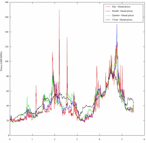
The second numerical experiment is performed using real dat The real da studied are electric power pri
(in m
a. ta ce
data taken from th ma data are
“spiky” a data made
n
he ere MWh), ed
e for
o o
e UK electricity rket. These sset prices. The time series studied is of the observatio times
0< <1 2< < n= 1395 < ,
t t t t (days), and of t
set price Si observed at time ti, wh is
Day-Ahead price, i= , , . n Excluding week-end days
and holidays this data time series corresponds to more than 5 years of daily observations going from January 5, 2004 to July 10, 2009. Remind that GBP means Great Britain Pound and that MWh means Mega-Watt/hour.
Moreover the data time series studied in correspondence of each spot price contains a series of forward prices associated to it for a variety of delivery periods. These prices include: forward price 1 month deep in the future (Month-Ahead price), forward price 3 months deep in the
future (Quarter-Ahead price), forward price 4 months
deep in the future (Season-Ahead price), forward price 1
year deep in the future (One Year-Ahead price). These
forward prices are observed each day ti and the forward
prices observed at time ti are associated to the spot
price Si, i= 0,1, ,1395. The spot and the forward
prices contained in the data time series mentioned above are shown in Figure 3.
The observed electric power prices generate data time series with a complicated structure. The stochastic dyna- mical system studied in this paper does not pretend to fully describe the properties of the electric power prices. Indeed it is able to model only one property of these pr
0 =
spiky as
the daily electric power spot price (GBP/ i
S
nam
0,1
, se o
the first ob
ices: the presence of spikes. In addition the electricity prices have many other properties, for example, they are mean reverting and have well defined periodicity, that is they have diurnal, weekly and seasonal cycles. A lot of specific models incorporating (some of) these features are discussed in the literature example [10].
Figure 3. The UK electric power price data.
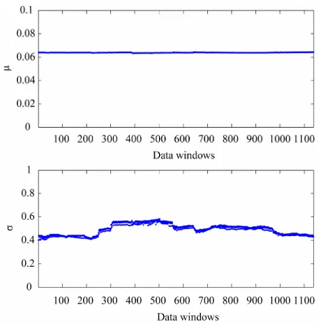
moving the window along the data are shown in Figures 4 and 5. In Figures 4 and 5 the abscissa represents the data windows used to reconstruct the model parameters numbered in ascending order according to the order in time of the first day of the window. Figures 4 and 5 show that the model parameters, with the exception of
,
are approximately constant functions of the data ow. The parameter
wind reconstructed shown in Figure 5 is a piecewise constant function. These findings support the idea that the model and the formulation of the calibration problem presented respectively in Sections 2 and 3 are adequate to interpret the data. In fact they
establish a stable relationship between the data and the model parameters as shown in Figures 4 and 5.
Figure 4. Reconstruction of the parameters of the Black- Scholes model: μ, σ.
Figure 5. Reconstruction of the parame e spikes: a, b, λ.
ele
ia
titatively the results shown in Figures 6-8 and gives the ters used to model th
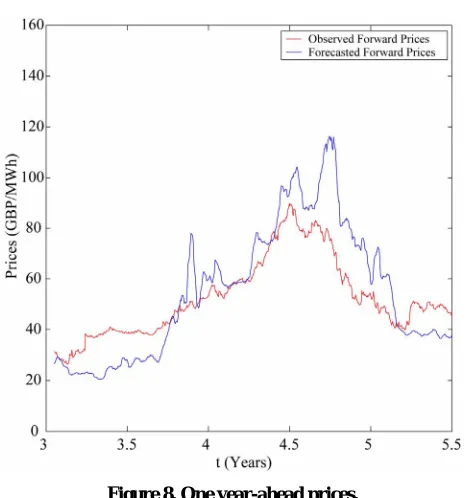
calculate the forecasted forward prices associated to the spot prices of the data time series not included in the data window mentioned above used in the calibration problem. In Figures 6-8 the forward electric power prices fore- casted are shown and compared to the observed forward ctric power prices. In Figures 6-8 the abscissa is the day of the spot price assoc ted to the forward prices computed. The abscissa of Figures 6-8 is coherent with the abscissa of Figure 3. Table 1 summarizes quan-
[image:11.595.307.537.165.575.2]Figure 6. Month-ahead prices.
Figure 7. Quarter-ahead prices.
ices with th
formulation of the calibration problem and its numerical average relative error eforward prices committed using the forecasted forward prices, that is the average relative error committed approximating the observed forward pr
e forecasted forward prices. Table 1 and Figures 6-8 show the high quality of the forecasted forward prices answering the second question posed about the analysis of the data time series in the affirmative.
[image:11.595.58.288.350.576.2]on Power with Scaling Spikes,” Nonlinear Analysis: Hy-brid Systems, Vol. 2, No. 2, 2008, pp. 285-304.
doi:10.1016/j.nahs.2006.05.002
[3] F. Mariani, G. Pacelli and F. Zirilli, “Maximum Likeli-hood Estimation of the Heston Stochastic Volatility Mo- del Using Asset and Option Prices: An Application of Nonlinear Filtering Theory,” Optimization Letters, Vol. 2, No. 2, 2008, pp. 177-222.
doi:10.1007/s11590-007-0052-7
[4] L. Fatone, F. Mariani, M. C. Recchioni and F. Zirilli, “Maximum Likelihood Estimation of the Parameters of a System of Stochastic Differential Equations that Models the Returns of the Index of Some Classes of Hedge Funds,” Journal of Inverse and Ill Posed Problems, Vol. 15, No. 5, 2007, pp. 493-526.doi:10.1515/jiip.2007.028
[5] L. Fatone, F. Mariani, M. C. Recchioni and F. Zirilli, “The Calibration of the Heston Stochastic Volatility Model Using Filtering and Maximum Likelihood Methods,” G. S. Ladde, N. G. Medhin, C. Peng and M. Sambandham, Eds., Proceedings of Dynamic Systems and Applications, Dy- namic Publishers, Atlanta, Vol. 5, 2008, pp. 170-181. [6] L. Fatone, F. Mariani, M. C. Recchioni and F. Zirilli,
“Calibration of a Multiscale Stochastic Volatility Model Us- ing European Option Prices,” Mathematical Methods in Eco- mics and Finance, Vol. 3, No. 1, 2008, pp. 49-61.
[7] L. Fatone, F. Mariani, M. C. Recchioni and F. Zirilli, “An
Explicitly ility Mo-
del: Optio nal of Futures
Markets, Vol. 29, No. 9, 2009, pp. 862-893.
[image:12.595.56.290.78.327.2]doi:10.1002/fut.20390 Figure 8. One year-ahead prices.
Table 1. Average relative errors of the forecasted forward electric power prices when compared to the observed for
e future
- ward prices.
Number of days in th
Solvable Multi-Scale Stochastic Volat n Pricing and Calibration,” Jour forward prices
e
30 (Month-Ahead prices) 0.0796
[8] L. Fatone, F. Mariani, M. C. Recchioni and F. Zirilli, “The Analysis of Real Data Using a Multiscale Stochastic Volatility Model,” European Financial Management, 2012, in press.
[9] P. Capelli, F. Mariani, M. C. Recchioni, F. Spinelli and F. Zirilli, “Determining a Stable Relationship between He- dge Fund Index HFRI-Equity and S&P 500 Behaviour, Using Filtering and Maximum Likelihood,” Inverse Pro- blems in Science and Engineering, Vol. 18, No. 1, 2010, pp. 93-109.
[10] C. R. Knittel and M. R. Roberts, “An Empirical Examina-tion of Restructured Electricity Prices,” Energy Econom-ics, Vol. 27, No. 5, 2005, pp. 791-817.
doi:10.1016/j.eneco.2004.11.005
90 (Quarter-Ahead prices) 0.1160
365 (One Year-Ahead prices) 0.2183
solution presented in this paper have the potential of be- ing tools of practical value in the analysis of data time series of spiky prices.
REFERENCES
[1] V. A. Kholodnyi, “Valuation and Hedging of European Contingent Claims on Power with Spikes: A Non-Marko- vian Approach,” Journal of Engineering Mathematics, Vol. 49, No. 3, 2004, pp. 233-252.
doi:10.1023/B:ENGI.0000031203.43548.b6
[2] V. A. Kholodnyi, “The Non-Markovian Approach to the Valuation and Hedging of European Contingent Claims
[image:12.595.58.286.380.447.2]