High Order Portfolio Optimization Problem with Transaction Costs

(1)

ISSN Online: 2152-7261 ISSN Print: 2152-7245

DOI: 10.4236/me.2019.106100 Jun. 12, 2019 1507 Modern Economy

High Order Portfolio Optimization Problem

with Transaction Costs

Xin Li, Peiai Zhang

*

Mathematics, Jinan University, Guangzhou, China

Abstract

This paper studies a high order moments portfolio optimization model with transaction costs. The model takes kurtosis as objective function and takes the skewness, variance, mean and transaction costs as constraints conditions. Since the optimization problem is of high order and non-convex, it brings some difficulties to the solution of the model. Therefore, this paper trans-forms the optimization problem into a semi-definite matrix optimization problem by using the moment matrix theory, and then solves it. Through the study of four risky assets in China’s securities market, it is found that transac-tion costs are significant parts in the study of portfolio model. In additransac-tion, sensitivity analysis shows that the kurtosis and skewness are positively corre-lated with the mean and variance invariant. When mean and skewness are constant, kurtosis and variance are positively correlated. When mean and skewness remain unchanged, the fourth order standard central moment and variance are negatively correlated.

Keywords

Portfolio, High Order Moment, Transaction Costs, Sensitivity Analysis

1. Introduction

The traditional Markowitz mean-variance model [1] is based on the fact that the utility function of investors is a quadratic function or that the return rate of asset portfolio obeys the normal distribution [2]. However, a plethora of empirical studies [3] show that the distributions of asset returns are not normally distribution, but tend to be of asymmetric, leptokurtic and heavy-tailed features. Therefore, it is not enough to study the mean and variance, but also to study high order moments (skewness and kurtosis) in investment decision.

Skewness and kurtosis are important factors to describe investment risk How to cite this paper: Li, X. and Zhang,

P.A. (2019) High Order Portfolio Optimi-zation Problem with Transaction Costs. Modern Economy, 10, 1507-1525.

https://doi.org/10.4236/me.2019.106100 Received: May 11, 2019

Accepted: June 9, 2019 Published: June 12, 2019

http://creativecommons.org/licenses/by/4.0/

(2)

DOI: 10.4236/me.2019.106100 1508 Modern Economy except variance. Among them, skewness is used to measure the skew direction and degree of statistical data distribution and to represent the asymmetric characteristics of statistical data. It is also used to represent the asymmetric characteristics of the probability density function of the assets yield. If the skewness is positive, it means that positive returns are easy to generate. If the skewness is negative, it means that the potential risk is greater than the potential benefit. Skewness is defined as the third-order standard central moment statistically,

( )

(

)

(

)

(

)

3

3 2 2

E r S r

E r µ

µ

 ₋ 

 

=

 ₋ 

 

where, r represents the assets yield, µ represents the expected return on risky assets.

Kurtosis is of a sharp peaks and fat tail character of the probability density function of the assets yield, compared with the normal distribution. If the kurtosis is 3, the density function of the assets yield is the same as the steepness of the normal distribution, that is, it has the same peak and tail characteristic. If the kurtosis is greater than 3, the density function of the assets yield is steeper than the normal distribution, that is, there are steeper peaks and thicker tails. If the kurtosis is less than 3, the density function of the assets yield is gentler than the normal distribution. Kurtosis is defined as the fourth-order standard central

moment statistically,

( )

(

)

(

)

(

)

4

2 2

E r K r

E r µ

µ

 ₋ 

 

=

 ₋ 

 

.

Many scholars have considered skewness and kurtosis in their studies. Jean Pierre Aubin and Hlne Frankowska [4] pointed out that investors prefer the yield with a large skewness (the third order central moment) and dislike the yield with a large kurtosis (the fourth order central moment). Yixuan Ran et al.

[5] considered the influence of skewness and kurtosis in their portfolio model and proposed the Grey Wolf Optimization algorithm to solve the problem. Amritansu Ray and Sanat Kumar Majumder [6] proposed a new non-Shannon fuzzy mean-variance-skewness-entropy model, which established a multi-objective non-linear portfolio model by maximizing mean and skewness and minimizing variance and cross-entropy. Mehmet Aksarayli and Osman Pala [7] proposed a multi-objective optimization model which concerned mean, variance, skewness, kurtosis and entropy simultaneously, and compared the out-of-sample per- formance of two entropy measures Shannon entropy and Gini-Simpson entropy in portfolio selection. Peng Shengzhi [8] established a portfolio model with kurtosis as the objective function and mean, variance and skewness as the constraint conditions, and solved it by semi-definite programming relaxation algorithm.

(3)

DOI: 10.4236/me.2019.106100 1509 Modern Economy portfolio problem with transaction costs. Arnott R D and Wagner W H [10], Enrico Angelelli [11] and others studied the impact of transaction costs in investment portfolios.Wang and Liu [12] studied the multi-period mean-variance portfolio problem with fixed transaction costs and proportional transaction costs. Suraj S. Meghwani and Manoj Thakur [13] incorporated transaction costs into the portfolio optimization model and formulated it as a three-objective problem, namely mean, variance and transaction costs. Atsushi Yoshimoto [14] studied the portfolio problem with variable transaction costs. Wei Chen et al. [15]

proposed a possibilistic mean-semi-absolute deviation portfolio model with V-shaped transaction costs, and solved it by FA-SA algorithm. Xue Deng et al.

[16] proposed the fuzzy mean-entropy portfolio models with transaction costs, and then sensitivity analysis of the objective function coefficients and constraint coefficients of the model.

Through the analysis of the above research, this paper takes transaction costs into account. In this paper, it is try to establish a portfolio model with kurtosis as the objective function and skewness, variance, mean and transaction costs as the constraints, then the model is transformed into a semi-definite matrix optimization problem by means of moment matrix theory, and then solved it. Moreover, this paper analyzed the impact of transaction costs on the portfolio, as well as the relationship between kurtosis and skewness, kurtosis and variance, fourth- order standard center moment and variance.

The rest of this paper is organized as follows. In Section 2, we present the portfolio optimization model with transaction costs. In Section 3, we describe the research methodology. In Section 4, this approach effectiveness is illustrated in experiments. Section 5 concludes the paper.

2. Model Description

2.1. Assumptions and Notations

In this section, assuming that in Chinese market without friction and not allowed to sell short. Then, The notation used in this article is illustrated. There are n risky assets,

(

)

T

1, , ,2 n

R= R R R is the assets yield vector,

(

)

T

1, , ,2 n

µ= µ µ µ is expected return vector of risk assets, x=

(

x x1, , ,2 xn

)

T is risk asset weight vector, T

1

n

P i i i

R =x R=

∑

− x R is portfolio return, µP =xTµ is Portfolio expected return, SP, VP and RP are respectively given skewness, variance and mean.

2.2. Model Establishment

(4)

DOI: 10.4236/me.2019.106100 1510 Modern Economy

(

)

(

)

(

)

(

)

(

)

(

)

(

)

4 2 2 3 3 2 2 2 T 1 min s.t. 1 0 P P P P P P P P P P P

P P P P

P P n i i i E R K E R E R S S E R

V E R V

x R x x µ µ µ µ µ µ µ =  ₋    =  ₋     ₋    = =  ₋      = _ − _= = = = ≥

∑

(1)

Because the variance of each stock is constant, therefore, this paper respectively using the third order central moment E r

(

₋

µ

)

3

  and fourth order center moment E r

(

₋

µ

)

4

  to describe of skewness and kurtosis, and Formula (1) can be reduced to:

(

)

(

)

(

)

4 3 2 T 1 min s.t. 1 0

P P P

P P P P

P P

n i i

i

K E R

S E R S

V E R V

x R x x µ µ µ µ µ =   = _ − _   = _ − _=   = _ − _= = = = ≥

∑

2.3. Establishment of Transaction Costs Function

Transaction costs can be divided into explicit costs and implicit costs. The explicit costs are also known as the fixed costs, which is the general name of various taxes such as procedure fee and stamp duty. Implicit costs refer to the indirect costs incurred in the course of securities transactions. This paper will start with explicit cost, and the most direct manifestation of explicit cost is stamp duty, transfer fee and brokerage commission. The charging rules [17] are as follows:

1) Stamp duty: It is charged at 1‰ of the transaction amount and is unilaterally levied, that is, it is charged separately to the seller according to the transaction amount of the stock transaction.

2) Transfer fee: It is charged at 0.02‰ of the transaction amount, but the fee is only paid when investors conduct Shanghai stock and fund transactions.

(5)

2.4. The Model with Transaction Costs

Assuming that the initial investment of the investor is 0, as this paper considers that short selling is not allowed in the market, so the investor’s investment ratio

i

x is not negative. Therefore, the total transaction costs function is

( )

T

i

C x =x

ω

where

(

)

T

1, , ,2 n

ω= ω ω ω , ωi represents a fixed proportion of the transaction amount, then the transaction costs function is a fixed proportional function of the investment amount [17], thus, the improved portfolio model with transaction costs can be expressed as:

(

)

(

)

(

)

4 3 2 T T 1 min s.t. 1 0

P P P

P P P P

P P

n i i

i

K E R

S E R S

V E R V

x x R

x x

µ

µ µ ω

=   = _ − _   = _ − _=   = _ − _= = − = = ≥

∑

(2)

2.5. Algebraic Representation of the First Four Order Moments of

the Portfolio Return Rate

The physics tensor operation is used to restate the variance, skewness and kurtosis of the portfolio yield, as follows [18][19]:

The variance of portfolio yield:

11 1 T T 2 1 1 1 n n n

P i j i j ij

n nn

V x x x x x M x

σ σ σ σ σ = =     = = _ _ =    

∑ ∑

where M2 =E R_

(

−

µ

)(

R−

µ

)

T_=

{ }

σ

_{ij n n}_× is an n n× order covariance matrix, its component is σij =E R_

(

i−µi

)

(

Rj−µj

)

_.

The skewness of portfolio yield:

(

)

T 3 1 1 1

n n n

P i j m i j m ijm

S =

∑ ∑ ∑

₌ ₌ ₌ x x x s =x M x x⊗

where

(

)(

) (

)

{ }

2

T T

3 _{ijm n n}

M =E R_ −

µ

R−

µ

⊗ R−

µ

_= s _× is an _{n n}_× 2 _order coskewness matrix, its component is sijm=E R

(

i−µi

)

(

Rj−µj

)

(

Rm−µm

)

,

⊗_{is the Kronecker product.} The kurtosis of the portfolio yield:

(

)

T 4 1 1 1 1

n n n n

P i j m l i j m l ijml

K =

∑ ∑ ∑ ∑

₌ ₌ ₌ ₌ x x x x k =x M x x x⊗ ⊗

where

(

)(

) (

)

{ }

3

T T T

4 _{ijml n n}

M ₌E R ₋

µ

R₋

µ

_⊗ R₋

µ

_⊗ R₋

µ

₌ k _×

  is an

3

n n× _{order cokurtosis matrix, its component is}

(

)

(

)

(

)(

)

ijml i i j j m m l l

k =E R_ −µ R −µ R −µ R −µ __.

(6)

( )

(

)

( )

(

)

( )

T 4 T 1 3 T 2 2 T T 3 4 1 min s.t. 1 0 P P P n i i i

p x x M x x x

g x x M x x S

g x x M x V

g x x x R

g x x

x µ ω = = ⊗ ⊗ = ⊗ = = = = − = = = ≥

∑

(3)

3. Method

According to Lasserre, Waki and Peng [8][20][21], the optimization problem is transformed into the linear matrix inequality optimization problem by using the moment matrix theorem, and then transformed it into a semi-definite matrix programming problem.

When

( )

T

(

)

4

1 1 1 1

n n n n

i j m l ijml

i j m l

p x x M x x x

x x x x k p xα

α α = = = = = ⊗ ⊗ = =

∑ ∑ ∑ ∑

∑

(4)

where, 1 2

1 2 nn

xα =x xα α xα , max

∑

n_i₌₁α_i =4.

The vector

(

2 2 4 4

)

1 2 1 1 2 1 1

1, , , , , ,x x x x x x_n , , x x_n, , , , , , x_n x x_n is the basis of the fourth-order polynomial p x

( )

, and p=

{ }

pα is the coefficient vector of

the basis components in p x

( )

. When

(

)

{

}

(

)

(

)

{

}

T T T T

3 2

1

T T

1 3 2 3

T T

3 2 4 2

T T T T

5 6

7 1 8 1

: , , ,

1, 0

: 0, 0,

0, 0,

1 0, 1 0, 0

n

P P P

n i i i n P P P P P P n n

i i i

i i

K x R x M x x S x M x V x x R

x x

x R h x M x x S h x M x x S

h x M x V h x M x V

h x x R h x x R

h x h x x

µ ω

µ ω µ ω

= = = = ∈ ⊗ = = − = = ≥ = ∈ = ⊗ − ≥ = − ⊗ + ≥ = − ≥ = − + ≥ = − − ≥ = − + + ≥ = − ≥ = − + ≥ ≥

∑

Theorem 1. [20] The P_K min_{x K}∈ p x

( )

and pK minµ∈P K( )

∫

_Kp x

( )

d

µ

are equivalent, that is, 1) infPK =infpK.

2) If x∗_{is a global minimizer of}

K

P , then µ∗:=δ_x∗ is a global minimizer

of pK.

3) If x∗_{is the unique global minimizer of}

K

P , then µ∗:=δ_x∗ is the unique

global minimizer of pK.

According to the theorem 1, Formula (3) can be converted into the following problem:

( )

(7)

DOI: 10.4236/me.2019.106100 1513 Modern Economy space to make

_∫

_Kp x

( )

dµ optimal.

From Formula (4), we can get

( )

d d

(

d

)

Kp x K p x p Kx p y

α α

α α α α

α α α

µ=

∑

µ=

∑

µ =

∑

∫

(6)

where, y _Kxαd

α =

∫

µ is the α-order moment of the probability measure µ.

Thus, the Formula (5) is transformed into the following problem:

{ }

min _y_α∈Γ

∑

αp yα α

The objective function becomes a linear function composed of a sequence of moments, which simplifies the problem.

The characteristics of

{ }

yα are described as below definitions.

Define 1 [22]: Matrix

( )

( ) ( )

000 0 100 0 010 0

100 0 200 0 110 0

010 0 110 0 020 0

2 s t

t

s t s t

y y y y

y y y

M y y y y

y y

 

 

=_ _

 

 

where, t is the degree of the objective function, and s t

( )

is the dimension of the basis of the objective function.

Define 2: M qyt

( )

is a matrix composed of components

( )( )

, _{ _{( )}_, _}

t r i j

M qy i j =

∑

q yβ +γ

where β

( )

i j, _{indicates the lower subscript of each component} yβ of M yt

( )

, and qr represents the coefficient corresponding to each component of the function q x

( )

.

Theorem 2. [8] If q x

( )

is a polynomial with a degree of 2d or 2d−1_and

( )

{

: 0

}

Q= x q x ≥ _{, then} M y_t

( )

0, M_{t d}−

(

q y∗

)

0.

According to the analysis, the Formula (3) can be transformed into the following semi-definite matrix optimization problem.

( )

(

)

T

min

s.t. 0

0 1,2, ,8

j t

t d j

p y M y

M h y

j

− ∗

=



 (7)

where, t≥max

(

d d0, , ,1 d8

)

.

4. Experimental Analysis

(8)

DOI: 10.4236/me.2019.106100 1514 Modern Economy Guotaian CSMAR database. The data needs to be preprocessed before the model is solved.

4.1. Sample Data Analysis

In order to simplify the problem, the risk-free assets are ignored, and the return on investment is based on the logarithmic returns, Rij =ln

(

A Aj j−1

)

, where i is

the i-th stock and j is the j-th day, Aj indicates the closing price of j-th day.

4.1.1. Calculate the Expected Rate of Return for Stock i

( )

i E Ri

µ =

Use the Excel to get the expected return on the four stocks, as shown in the following Table 1.

4.1.2. Stock Variance, Third-Order Standard Center Moment, Excess Kurtosis (Fourth-Order Standard Center Moment Minus 3), Skewness, Kurtosis, Jarque-Bera Statistic

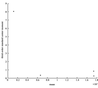
[image:8.595.209.533.354.643.2]

A scatter plot of the mean and third-order standard central moment and a scatter plot of the mean and excess kurtosis are given in Table 2, as shown in the following Figure 1.

[image:8.595.206.541.688.737.2]

Figure 1. Scatter plot of mean and third-order standard central moment.

Table 1. Expected rate of return for each stock.

stocks Shenzhen Energy Western Securities Baiyun Airport Guangzhou Port

i

(9)

[image:9.595.212.537.203.482.2]

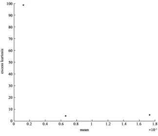
DOI: 10.4236/me.2019.106100 1515 Modern Economy From Figure 1, we can get the third-order standard central moment of the four stocks are positive, and none of them are zero, indicating that the four stocks have certain asymmetry. From Figure 2, we can get the excess kurtosis of the four stocks are all positive, indicating that they have certain characteristics of sharp peaks and fat tail, especially the third stock, baiyun airport. The Jarque- Bera statistic of the four stocks’ returns are greater than the critical value of 0.5% of the

_χ

2

( )

₂ _{distribution. Then we can confirm the non-normal distribution} characteristics of the return rates on the four stocks.

Figure 2. Scatter plot of mean and excess kurtosis.

Table 2. Mean, Variance, Third-order standard center moment, Excess kurtosis, Skewness, Kurtosis, Jarque-Bera statistic for each stock.

stocks Shenzhen _Energy _SecuritiesWestern _AirportBaiyun Guangzhou _Port

Mean 0.00065955 0.00173903 0.00011836 0.00173632

Variances 0.00010518 0.00039679 0.00083951 0.00046760

Third-order standard

center moments 0.34597184 0.83363682 8.04344754 0.26292693

Excess kurtosis 4.37482549 5.55668050 98.58424447 5.24389392

Skewness 0.00000037 0.00000655 0.00019445 0.00000264

Kurtosis 0.00000008 0.00000134 0.00007101 0.00000179

[image:9.595.212.539.537.736.2]

(10)

4.2. Solve the Problem

4.2.1. Solution of Portfolio Optimization Problem without Transaction Costs

According to the sample data, we will study the above portfolio model without transaction costs. Firstly, we can set RP =0.00005332, VP =0.00019227 and

0.00000510 P

S = _{, Formula (3) is concretized into the following optimization}

problem:

( )

4 4 4

1 2 3

4 2 2 2 2

4 1 2 3 4

2 2 2 2 2 2

1 3 1 4 2 3

2 2 3 3

2 4 1 2 1 3

min 0.00000008 0.00000134 0.00007101 0.00000179 0.00000090 0.00000177 0.00000038 0.00000131 0.00000166 0.00000431 0.00000031 0.00000015 0.00

p x x x x

x x x x x

x x x x x x

= + +

+ + +

+ 3 3 3

1 4 1 2 2 3

000039x x +0.00000151x x +0.00000174x x

3 3 3

2 4 1 3 2 3

3 3 3

3 4 1 4 2 4

3 2 2

3 4 1 2 3 1 2 4

2 2 2

1 2 3 1 2 4 1 3

0.00000314 0.00000366 0.00000442 0.00000587 0.00000210 0.00000321 0.00000143 0.00000074 0.00000169

0.00000176 0.00000363 0.00000077

x x x x x x

x x x x x x x x

x x x x x x x x

+ − +

+ + +

+ + + ₄

2 2 2

1 2 3 1 3 4 1 2 4

0.00000091 0.00000084 0.00000388

x

x x x x x x x x x

+ + +

2 2 2

1 3 4 2 3 4 2 3 4 2

2 3 4 1 2 3 4

0.00000184 0.00000386 0.00000265

0.00000372 0.00000303

x x x x x x x x x

x x x x x x x

+ + +

+ +

( )

3 3 3

1 1 2 3

3 2 2

4 1 2 1 3

2 2 2

1 4 1 2 2 3

2 2 2

2 4 1 4 2 4

s.t. 0.00000037 0.00000655 0.00019445 0.00000264 0.00000441 0.00000089 0.00000553 0.00001057 0.00000985 0.00002373 0.00001107 0.00002142

g x x x x

x x x x x

x x x x x x

= + +

+ + +

2 2 2

3 4 1 3 2 3

2

3 4 1 2 3 1 3 4 1 2 4 2 3 4

0.00000555 0.00000675 0.00001391 0.00001557 0.00000668 0.00000571 0.000020801 0.000014431 0.00000510

x x x x x x

x x x x x x x x

x x x x x x

+ − +

+ + +

+ + =

( )

2 2 2

2 1 2 3

2

4 1 2 1 3

1 4 2 3 2 4

3 4

0.00010518 0.00039679 0.00083951 0.00046760 0.00022167 0.00009557 0.00024047 0.00021917 0.00039333 0.00019957 0.00019227

g x x x x

x x x x x

x x x x x x

x x = + + + + + + + + + =

( )

3 1 2 3

4

4 1 2 3 4

0.00065955 0.00173903 0.00011836 0.00173632 0.00005332

1 0, 1,2,3,4

i

g x x x x

x

g x x x x x

x i = + + + = = + + + = ≥ = (8)

According to Formula (8), the basis vector of the objective function p x

( )

is

(

2 2 4 4

)

1 2 3 4 1 1 2 1 3 1 4 4 1 4

1, , , , , ,x x x x x x x x x x x, , , , , , , , x x x (9) From Formula (6), Formula (9) can be converted into the following form:

( ) (

0000, 1000, 0100, 0010, , 0004

)

(11)

DOI: 10.4236/me.2019.106100 1517 Modern Economy According to Formula (8), constraints can be converted into the following form:

( )

1 1 2 1 3 2 4 2 0.00000510 0 0.00000510 0 0.00019227 0 0.00019227 0

h g x

= − ≥ = − + ≥ = − ≥ = − + ≥

( )

5 3 6 3 7 4 8 4 0.00005332 0 0.00005332 0 1 0 1 0

h g x

= − ≥

= − + ≥

= − ≥

= − + ≥

According to Formula (7), Formula (8) can be converted into the following form:

( )

(

)

(

)

(

)

T 4 2 1 2 2 3 3 min s.t. 0 0 0 0 p y M y M h y M h y M h y ∗ ∗ ∗    

(

)

(

)

(

)

(

)

(

)

3 4 3 5 3 6 3 7 3 8 0 0 0 0 0

M h y M h y M h y M h y M h y ∗ ∗ ∗ ∗ ∗     

Using MATLAB to solve the problem, minimize the kurtosis of the optimal portfolio is obtained:

(

) (

T

)

T

1, , ,2 3 4 0.2870,0.2160,0.2210,0.2760

x= x x x x =

From the results, we can see that only by investing 28.70% of the total investment amount in Shenzhen Energy, 21.60% in Western Securities, 22.10% in Baiyun Airport and 27.60% in Guangzhou Port, so that the minimum kurtosis is 0.00000040.

After studying the case without transaction costs, we will continue to study the above portfolio optimization problem when considering transaction costs.

4.2.2. Solution of Portfolio Optimization Problem with Transaction Costs

According to the sample data, Formula (3) is concretized into the following optimization problem:

( )

4 4 4

1 2 3

4 2 2 2 2

4 1 2 3 4

2 2 2 2 2 2

1 3 1 4 2 3

2 2 3 3

2 4 1 2 1 3

min 0.00000008 0.00000134 0.00007101 0.00000179 0.00000090 0.00000177 0.00000038 0.00000131 0.00000166 0.00000431 0.00000031 0.00000015 0.0

p x x x x

x x x x x

x x x x x x

′ = + +

+ + +

+ 3 3 3

1 4 1 2 2 3

(12)

3 3 3

2 4 1 3 2 3

3 3 3

3 4 1 4 2 4

3 2 2

3 4 1 2 3 1 2 4

2 2 2

1 2 3 1 2 4 1 3

0.00000314 0.00000366 0.00000442 0.00000587 0.00000210 0.00000321 0.00000143 0.00000074 0.00000169

0.00000176 0.00000363 0.00000077

x x x x x x

x x x x x x x x

x x x x x x x x

+ − +

+ + +

+ + + ₄

2 2 2

1 2 3 1 3 4 1 2 4

0.00000091 0.00000084 0.00000388

x

x x x x x x x x x

+ + +

2 2 2

1 3 4 2 3 4 2 3 4 2

2 3 4 1 2 3 4

0.00000184 0.00000386 0.00000265

0.00000372 0.00000303

x x x x x x x x x

x x x x x x x

+ + +

+ +

( )

3 3 3

1 1 2 3

3 2 2

4 1 2 1 3

2 2 2

1 4 1 2 2 3

2 2 2

2 4 1 4 2 4

s.t. 0.00000037 0.00000655 0.00019445 0.00000264 0.00000441 0.00000089 0.00000553 0.00001057 0.00000985 0.00002373 0.00001107 0.00002142

g x x x x

x x x x x

x x x x x x

′ = + +

+ + +

2 2 2

3 4 1 3 2 3

2

3 4 1 2 3 1 3 4 1 2 4 2 3 4

0.00000555 0.00000675 0.00001391 0.00001557 0.00000668 0.00000571 0.000020801 0.000014431 0.00000510

x x x x x x

x x x x x x x x

x x x x x x

+ − +

+ + +

+ + =

( )

2 2 2

2 1 2 3

2

4 1 2 1 3

1 4 2 3 2 4

3 4

0.00010518 0.00039679 0.00083951 0.00046760 0.00022167 0.00009557 0.00024047 0.00021917 0.00039333 0.00019957 0.00019227

g x x x x

x x x x x

x x x x x x

x x ′ = + + + + + + + + + =

( )

3 1 2 3

4

4 1 2 3 4

0.00034045 0.00073903 0.00090164 0.00073632 0.00005332

1 0, 1,2,3,4

i

g x x x x

x

g x x x x x

x i ′ = − + − + = ′ = + + + = ≥ = (10)

According to Formula (10), the constraints can be converted into the following form:

( )

1 1 2 1 3 2 4 2 0.00000510 0 0.00000510 0 0.00019227 0 0.00019227 0

h g x

′= ′ − ≥ ′= − ′ + ≥ ′= ′ − ≥ ′= − ′ + ≥

( )

5 3 6 3 7 4 8 4 0.00005332 0 0.00005332 0 1 0 1 0

h g x

′= ′ − ≥

′= − ′ + ≥

′= ′ − ≥

′= − ′ + ≥

(13)

(

)

(

)

(

)

(

)

(

)

3 4

3 5

3 6

3 7

3 8

0 0 0 0 0

M h y M h y M h y M h y M h y ′ ∗ ′ ∗ ′ ∗ ′ ∗ ′ ∗

    

Similarly, using MATLAB to solve it, minimize the kurtosis of the optimal portfolio is obtained:

(

) (

T

)

T

1, , ,2 3 4 0.2740,0.2259,0.2340,0.2661

x= x x x x =

From the results, we can see that only by investing 27.40% of the total investment amount in Shenzhen Energy, 22.59% in Western Securities, 23.40% in Baiyun Airport and 26.61% in Guangzhou Port, so that the minimum kurtosis is 0.00000045.

4.2.3. Summary

Without transaction costs, the investor takes 28.70% of the total investment amount to invest in Shenzhen Energy, 21.60% to invest in Western Securities, 22.10% to invest in Baiyun Airport and 27.60% to invest in Guangzhou Port. At this time, it can be concluded that the minimum kurtosis of the investment portfolio is 0.00000040. When transaction costs are taken into account, investors invest 27.40% of the total investment amount in Shenzhen Energy, 22.59% in Western Securities, 23.40% in Baiyun Airport and 26.61% in Guangzhou Port. At this time, the minimum kurtosis of the investment portfolio is 0.00000045. In both cases, although Shenzhen Energy has the largest proportion of investment, followed by Guangzhou Port and finally Western Securities, the proportion of investment in the four stocks is different. In addition, according to the analysis of the transaction costs function, the transaction cost accounts for 1‰ of the investment amount. When the investment amount increases, the transaction costs will increase relatively. Therefore, in the investment process, the impact of transaction costs cannot be ignored.

4.3. Sensitivity Analysis of the Relationship between Kurtosis,

Skewness and Variance

In this section, we will give the relationship between kurtosis and skewness, kurtosis and variance, and the relationship between fourth-order standard central moment and variance, then further verify the effectiveness of the above solution.

4.3.1. Sensitivity Analysis of the Relationship between Kurtosis and Skewness

(14)

[image:14.595.222.526.75.336.2]

Figure 3. Relationship between skewness and kurtosis.

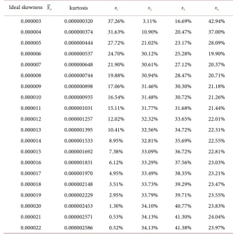
Table 3. The optimal solution and the change of optimal portfolio kurtosis with SP.

Ideal skewness SP kurtosis x1 x2 x3 x4

[image:14.595.204.538.389.726.2]

(15)

DOI: 10.4236/me.2019.106100 1521 Modern Economy portfolio are positively correlated. Under the mean and variance of the portfolio unchanged, the kurtosis of the optimal portfolio increases with the increase of the skewness, which means that investors want to increase the skewness of the portfolio and need to take more risk of kurtosis.

4.3.2. Sensitivity Analysis of the Relationship between Kurtosis and Variance

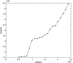
In the previous section, we analyzed the relationship between kurtosis and variance. In this section, we will continue to analyze the relationship between kurtosis and variance and the relationship between the fourth order standard central moment and variance. Firstly, we can set RP =0.00005332 and

0.00000510 P

[image:15.595.226.525.450.706.2]

S = _{, then continuously adjust the ideal variance}V_P, and we can obtain a series of the optimal solution and the kurtosis of the optimal portfolio, as shown in Table 4. From Table 4, the relationship of variance and the optimal portfolio kurtosis can be plotted in Figure 4, and the relationship of variance and fourth-order standard central moment can be drawn in Figure 5. From

Figure 4, we can see that the kurtosis and variance of the optimal portfolio are positively correlated. When the portfolio’s mean and skewness constant, the variance increases and the kurtosis of the optimal portfolio is also increase. Since the calculation of the fourth-order standard central moment K r

( )

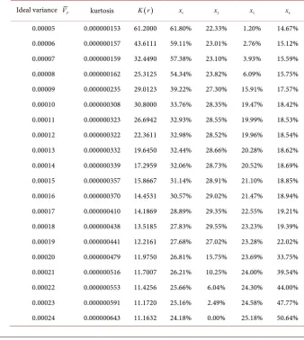
is related to the variance, we also need to study the relationship between the variance and the fourth-order standard central moment. As shown in Figure 5, the variance is negatively correlated with the fourth-order standard center moment, which means that the fourth-order standard center moment decreases with increasing variance when the portfolio mean and skewness are constant.

(16)

[image:16.595.230.519.66.309.2]

Figure 5. Relationship between variance and fourth-order standard center moment.

Table 4. The optimal solution and the change of optimal portfolio kurtosis with VP.

Ideal variance VP kurtosis K r( ) x1 x2 x3 x4

[image:16.595.198.537.362.741.2]

(17)

5. Conclusions

In this paper, we study the portfolio model with skewness, kurtosis and transac-tion costs. This model takes kurtosis as the objective functransac-tion and takes skew-ness, variance, mean and transaction costs as the constraint conditions. Because of non-convexity and high order of the objective function, this paper, based on Lasserre and Waki’s research, transform the optimization problem into a semi- definite matrix optimization problem for solving. This method can effectively avoid the non-convexity and high order moment.

This paper selected two stocks of Shenzhen Stock Exchange, Shenzhen Energy (000027) and Western Securities (002673), and two stocks of Shanghai Stock Exchange, Baiyun Airport (600004) and Guangzhou Port (601228). By the ex-ample, we can get that the transaction costs would make the investment ratio of the four stocks different, in the case of other conditions unchanged. When we study the portfolio problem, the transaction costs cannot be ignored. In addi-tion, we obtain the relationship between the kurtosis of the optimal portfolio and the variance, the relationship between the kurtosis of the optimal portfolio and the skewness and the relationship between the fourth-order standard center moment and the variance, through Sensitivity analysis. More accurately, the kurtosis and skewness of the portfolio are positively correlated, when the mean and variance of the portfolio are constant. Moreover, the kurtosis and variance of the portfolio are also positively correlated, when the mean and skewness of the portfolio are constant. Since the calculation of the fourth-order standard central moment is related to the variance, we also need to study the relationship between the fourth-order standard central moment and the variance. When the portfolio mean and skewness are constant, the fourth-order standard central moment decreases as the variance increases.

Acknowledgements

I would like to thank my parents for their encouragement and all the classmates who care about me for their support.

Conflicts of Interest

The authors declare no conflicts of interest regarding the publication of this pa-per.

References

[1] Markowitz, H. (1952) Portfolio Selection. Journal of Finance, 7, 77-91.

https://doi.org/10.1111/j.1540-6261.1952.tb01525.x

[2] Liu, L. (2004) A New Foundation for the Mean-Variance Analysis. European Jour-nal of OperatioJour-nal Research, 158, 229-242.

https://doi.org/10.1016/S0377-2217(03)00301-1

[3] Adams, R. (1975) Sobolev Space. Academic Press, New York.

(18)

DOI: 10.4236/me.2019.106100 1524 Modern Economy [5] Ren, Y., Ye, T., Huang, M. and Feng, S. (2004) Gray Wolf Optimization Algorithm for Multi-Constraints Second-Order Stochastic Dominance Portfolio Optimization. Algorithms, 11, 72.

[6] Ray, A. and Majumder, S.K. (2018) Objective Mean-Variance-Skewness Model with Burg’s Entropy and Fuzzy Return for Portfolio Optimization. Application Article, 55, 107-133.https://doi.org/10.1007/s12597-017-0311-z

[7] Aksarayli, M. and Pala, O. (2018) A Polynomial Goal Programming Model for Portfolio Optimization Based on Entropy and Higher Moments. Expert Systems with Applications, 94, 185-192.https://doi.org/10.1016/j.eswa.2017.10.056

[8] Peng, S.Z. (2016) Research on Portfolio Optimization Based on High Order Mo-ment.

[9] Chen, A.H.Y., Jen, F.C. and Zionts, S. (1971) The Optimal Portfolio Revision Policy. The Journal of Business, 44, 51-61.https://doi.org/10.1086/295332

[10] Arnott, R.D. and Wagner, W.H. (1986) Assert Pricing and the Bidask Spread. Jour-nal of Financial Economics, 17, 223-249.

https://doi.org/10.1016/0304-405X(86)90065-6

[11] Angelelli, N., Mansini, R. and Speranza, M.G. (2008) A Comparison of MAD and CVaR Models with Real Features. Journal of Banking Finance, 32, 1188-1197.

https://doi.org/10.1016/j.jbankfin.2006.07.015

[12] Wang, Z. and Liu, S. (2013) Multi-Period Mean-Variance Portfolio Selection with Fixed and Proportional Transaction Costs. Journal of Industrial and Management Optimization, 9, 643-657.https://doi.org/10.3934/jimo.2013.9.643

[13] Meghwani, S.S. and Thakur, M. (2018) Multi-Objective Heuristic Algorithms for Practical Portfolio Optimization and Rebalancing with Transaction Cost. Applied Soft Computing, 67, 865-894.https://doi.org/10.1016/j.asoc.2017.09.025

[14] Yoshimoto, A. (1996) The Mean-Variance Approach to Portfolio Optimization Subject to Transaction Costs. Journal of the Operations Research Society of Japan, 39, 99-117.https://doi.org/10.15807/jorsj.39.99

[15] Chen, W., Wang, Y. and Mehlawat, M.K. (2018) A Hybrid FA-SA Algorithm for Fuzzy Portfolio Selection with Transaction Costs. Annals of Operations Research, 269, 129-147.https://doi.org/10.1007/s10479-016-2365-3

[16] Deng, X., Zhao, J. and Li, Z. (2018) Sensitivity Analysis of the Fuzzy Mean-Entropy Portfolio Model with Transaction Costs Based on Credibility Theory. International Journal of Fuzzy Systems, 20, 209-218.https://doi.org/10.1007/s40815-017-0330-1 [17] Li, X.P. and Wen, J.E. (2016) Modeling and Algorithm of Practical Asset Allocation

Optimization Including Transaction Cost. Mathematical Modeling and Its Applica-tion, 3, 45-52.

[18] De Athayde, G.M. and Flres Jr., R.G. (2004) Finding a Maximum Skewness Portfo-lio—A General Solution to Three-Moments Portfolio Choice. Journal of Economic Dynamics and Control, 28, 1335-1352.

https://doi.org/10.1016/S0165-1889(02)00084-2

[19] De Athayde, G.M. and Flores Jr., R.G. (2003) Incorporating Skewness and Kurtosis in Portfolio Optimization: A Multidimensional Efficient Set. In: Satchell, S. and Scowcroft, A., Eds., Advances in Portfolio Construction and Implementation, El-sevier, Amsterdam, 243-257.https://doi.org/10.1016/B978-075065448-7.50011-2 [20] Lasserre, J.B. (2001) Global Optimization with Polynomials and the Problems of

Moments. SIAM Journal on Optimization, 11, 796-817.

https://doi.org/10.1137/S1052623400366802

(19)

DOI: 10.4236/me.2019.106100 1525 Modern Economy Semi-Definite Programming Relaxations for Polynamial Optimization Problems with Structured Sparsity. SIAM Journal on Optimization, 17, 218-242.