Polarization Filtering Method for Suppressing Surface Wave in Time Frequency Domain

(1)

ISSN Online: 2156-8367 ISSN Print: 2156-8359

DOI: 10.4236/ijg.2019.104028 Apr. 30, 2019 481 International Journal of Geosciences

Polarization Filtering Method for Suppressing

Surface Wave in Time-Frequency Domain

Xiaoming Yang

1

, Yang Gao

2

, Wenzhong Zhang

1

, Yanchun Wang

1*

, Meihua Lan

3

1_{School of Geophysics and Information Technology, China University of Geosciences 1, Beijing, China}

2_{Key Laboratory of Coal Resources Exploration and Comprehensive Utilization, Ministry of Land and Resources, Xi’an, China} 3_{Information Center Computer Office, Daqing Drilling & Exploration Engineering Corporation No.1 Geo-Logging Company,} Daqing, China

Abstract

In order to suppress the surface wave in three-component seismic explora-tion, according to the polarization characteristics of body wave and surface wave, a time-frequency domain polarization filtering method based on wave-let transform was studied. A covariance matrix was constructed in the time-frequency domain for the three-component seismic data, measured the polarization parameters of seismic waves. Combining the corresponding ei-genvalues and eigenvectors of the matrix, the elliptic rate and elevation angle were used as constraints, and the polarization filter function was built to sep-arate the surface waves. The sepsep-arated surface waves were inversely trans-formed and then were adaptively subtracted from the original records. After the polarization filtering suppressed the surface wave, the signal-to-noise ra-tio of the converted wave was effectively improved. It laid a good foundara-tion for the next seismic data processing and seismic exploration development. The actual data processing results show that the method can effectively ex-tract surface waves from three-component seismic records and avoid the in-terference of surface waves on seismic signals.

Keywords

Three-Component Seismic Data, Surface Wave, Polarization Filtering, Adaptation

1. Introduction

In seismic exploration, surface waves are typical regular disturbances, and sur-face waves are usually suppressed based on the apparent velocity and frequency How to cite this paper: Yang, X.M., Gao,

Y., Zhang, W.Z., Wang, Y.C. and Lan, M.H. (2019) Polarization Filtering Method for Suppressing Surface Wave in Time-Frequency Domain. International Journal of Geos-ciences, 10, 481-490.

https://doi.org/10.4236/ijg.2019.104028

Received: March 13, 2019 Accepted: April 27, 2019 Published: April 30, 2019

http://creativecommons.org/licenses/by/4.0/

(2)

DOI: 10.4236/ijg.2019.104028 482 International Journal of Geosciences difference between the surface wave and the effective wave. In the three-component seismic exploration, the converted wave energy is weak. In the shallow layer, the converted wave apparent velocity overlaps with the surface wave. In the deep layer, the converted wave frequency overlaps with the surface wave. Therefore, the converted wave is greatly disturbed by surface waves. Ac-cording to the different polarization characteristics between body wave and sur-face wave, a polarization filtering method is studied to suppress the sursur-face wave.

Initially, Shimshoni and Smith separated the signals in natural and nuclear explosions according to the polarization characteristics of seismic waves [1]. Flinn calculated the three-component seismic data covariance matrix in a certain time window, constructed a series of polarization parameters that can describe the polarization characteristics of seismic waves, and separated the wave fields with different polarization characteristics. The disadvantage of this method is that it depends on the selection of window length, and the polarization parame-ters are not time-varying [2]. Samson proposed the concept of polarization coef-ficient, which provides a basis for designing various polarization filter factors. With the application of three-component technique in practice, geophysicists have developed a variety of polarization analysis techniques [3]. Benhama, Jur-kevics, Shieh C, Huang, Chen, Liu, etc. perform polarization analysis in the time domain and frequency domain [4]-[9]. Christoffersson proposed the maximum likelihood method [10]. Jackson et al. proposed the singular value decomposi-tion method [11]. Vidale, Rene, Stewart, Morozov, etc. developed instantaneous polarization analysis, etc. [12][13][14][15]. Huang Zhongyu and Gao Lin stu-died the three-component polarization analysis and its practical application [7]. Zhang Yufen and Zhou Jianxin analyzed the factors affecting filtering effect in the spatial direction [16]. Tatham et al. pointed out that due to the complexity of underground media, the use of the elliptic rate alone does not effectively sepa-rate the surface waves [17]. The above mentioned methods all use fixed time windows, so the effect of suppressing surface waves is not ideal.

(3)

DOI: 10.4236/ijg.2019.104028 483 International Journal of Geosciences

2. Method Principle

2.1. Wavelet Transform

The wavelet transform decomposes signals x(t) by telescopic translation in mul-ti-scales, and finally achieves the result that the time subdivision at high fre-quency and the frefre-quency subdivision at low frefre-quency [18].

( )

,

(

b a, ,

)

1 t b

( )

d

WT b a g x g x t t

a a +∞ _∗ −∞ −   = = _ _  

∫

(1)

Let

( )

, 1

b a t b

g t g

a a

−

 

= _ _

  (2) where WT b a

( )

, is the wavelet transformed signal; wavelet g(t) produces a “time-frequency” window that changes with frequency by stretching a and translation b, a is the frequency scale factor, b is the time factor, the symbol * in-dicates the conjugate complex number. The wavelet transform of seismic signals generally uses Morlet wavelets:

( )

2 2 0 2π 2 e e r if t _a

g t = − ₍₃₎

where e is a natural constant; i is an imaginary number; f0 is the center frequen-cy.

The data WT b a

( )

, can be recovered by the formula (4).

( )

1 1₂

( )

, d d

g

t b

x t g WT b a b a

c a a

+∞ −∞ −   = _ _  

∫

(4)

where

( )

2 0 d g g f c f f +∞

=

_∫

_, g f

( )

is the Fourier transform of wavelet g(t).

The scale factor a is related to the center frequency f0 of g(t) and can be related to the physical frequency by a = f0/f. The scale factor a can stretch the basic wavelet, the wavelet width is proportional to a, and the amplitude is proportion-al to 1/a, but the shape (area) of the wavelet remains unchanged. The larger the scale, the longer the wavelet function is in time. Then the wavelet function processes the longer part of the signal, and the low frequency characteristic of the signal is obtained. On the other hand, when the scale factor is smaller, the wavelet function only processes the shorter part of the signal, so the high fre-quency characteristic of the signal is obtained.

2.2. Parameters Calculation

For the three-component seismic signal ui(t) (i = x, y, z), its wavelet transform in the time-frequency domain is WT b ai

( )

, . When the time is b, its local approxi-mation can be expressed as W bi

(

+τ,a

)

, this can be expressed as formula (5) by the modulus and phase of the wavelet transform:

(

,

)

( )

, cos

( )

, arg

( )

,

i i i k

(4)

DOI: 10.4236/ijg.2019.104028 484 International Journal of Geosciences where Ωi

( )

b a, is the instantaneous frequency function of i component at scale

a and time b, it is defined as:

( )

, arg

( )

,

i b a ∂_b WT b ai

Ω =

∂ (6) In order to avoid numerical derivation, the wavelet g(t) and its derivative is used to obtain the exact equation of Ωi

( )

b a, .

( )

, Im

_{( )}

( )

,

, g i

i g

i

WT b a b a

WT b a ′

 

Ω = −  

 

  (7) where Im[.] represents the complex imaginary part.

Using the wavelet transform WT b ai

( )

, of three-component seismic data, we can construct a covariance matrix in the time-frequency domain.

( )

( ) ( ) ( )

, , , , , , , , , ,

xx xy xz

xy yy yz

xz yz zz

I b a I b a I b a

M b a I b a I b a I b a

I b a I b a I b a

    =         (8) Here

( )

_{( )}

( )

, , , , ,

, , , sinc ,

2 cos arg , arg ,

, ,

sinc , 2

cos arg , arg ,

k m

k m k m k m

k m

k m

k m k

b a b a

I b a WT b a WT b a T b a

WT b a WT b a

b a b a

T b a

WT b a WT b a µ

 Ω − Ω 



= _{× } _ _

  



× _ − _

Ω − Ω

 

+ _ _

 



× _ + __ −

 µm

(9)

where k, m = (x, y, z), μ is the mean of the k component in the time window:

( )

_{( )}

( )_{( )}

(

)

( )

( ) ( )

, 2 , 2 , 1

, , d

,

Re , sinc , , 2

T b a

k _{T b a} k

k m

k k

b a W b a

T b a

WT b a T b a b a

µ = ₋ +τ τ

= _ _ _ Ω _

∫

(10)

where Re(∙) represents a complex imaginary part, Sinc(∙) represents a singular function. T b a

( )

, is the adaptive time window length determined by the in-stantaneous frequency of time b and scale a. In fact, different components of the signal often have different instantaneous frequencies, so it is necessary to calcu-late an average time window T b a

( )

, by the instantaneous frequencies of mul-tiple components.

( )

,

_{( )}

6π

_{( )}

2π

_{( )}

, , , xyz ,

x y z av

N N

T b a

b a b a b a b a

= =

Ω + Ω + Ω Ω (11)

where N is a positive integer, N = 1 or 2; xyz av

Ω _{is the average of the} instantane-ous frequencies of the three components.

(5)

instantane-DOI: 10.4236/ijg.2019.104028 485 International Journal of Geosciences ous energy at each time-frequency point. Calculate its eigenvalues λi(i = 1, 2, 3;

λ1 > λ2 > λ3) and the corresponding eigenvector Vi. The instantaneous polariza-tion parameters in the time-frequency domain are derived from the results, and the energy magnitude and direction of the particle in the time window are de-scribed. For linearly polarized waves, the covariance matrix has only one non-zero eigenvalue, and the polarization direction of the seismic wave can be judged by the corresponding eigenvector. For seismic waves vibrating in one plane, the covariance matrix has two non-zero eigenvalues, which determine the polarization plane. In the actual data, the polarization direction exists in the en-tire 3 space, so the three eigenvalues are not zero. The largest eigenvalue λ1(b, a) corresponds to the eigenvector V1(V1,x, V1,y, V1,z) as the main eigenvector. Among the three eigenvalues, the seismic signal energy is focused on the largest eigenvalue.

The polarization parameters calculated from the eigenvalues and eigenvectors of the time-frequency domain covariance matrix are mainly as follow:

1) Instantaneous polarization vector Instantaneous main polarization vector

( )

( ) ( )

1

_{( )}

1

,

, ,

,

V b a

R b a b a

V b a λ

= ₍₁₂₎

Instantaneous intermediate polarization vector

( )

( ) ( )

2

_{( )}

2

,

, ,

,

s

V b a

r b a b a

V b a λ

= (13)

Instantaneous sub-polarization vector

( )

( ) ( )

3

_{( )}

3

,

, ,

,

V b a

r b a b a

V b a λ

= ₍₁₄₎

2) Ellipticity Primary ellipticity

( )

b a, r b as

( )

, R b a

( )

,

ρ

= (15)

Secondary ellipticity

( )

1 b a, r b a, r b as ,

ρ

= ₍₁₆₎

3) Dip angle

( )

(

( )

2

( )

2

( )

)

1, 1, 1,

, arctan x , y , z ,

b a V b a V b a V b a

δ = + (17)

4) Azimuth

( )

b a, arctan

(

V b a V b a1,y

( )

, 1,x

( )

,

)

α

= ₍₁₈₎

2.3. Filter Function

After analysis and testing, the ellipticity ρ

( )

b a, and dip angle

( )

b a, π 2

( )

b a,

(6)

DOI: 10.4236/ijg.2019.104028 486 International Journal of Geosciences effectively. This paper combines these two parameters to construct a filter func-tion.

( )

, e

( )

, i

( )

, , 0

WT b a =F b a WT b a a>

( )

, 1

( )

,

( )

,

0 others

e

b a P b a P

F b a _{= } ρ ∈ ρ θ ∈ θ



且

(19)

where Fe is the polarization filter function applied to each of the original com-ponents, Pρand Pθdefine the range of variation of ρ and θ. Set the appropriate Pρ and Pθto obtain the desired output. In the actual data processing, the parameters were tested multiple times to ensure that the surface wave was suppressed prop-erly.

3. Filtering Steps

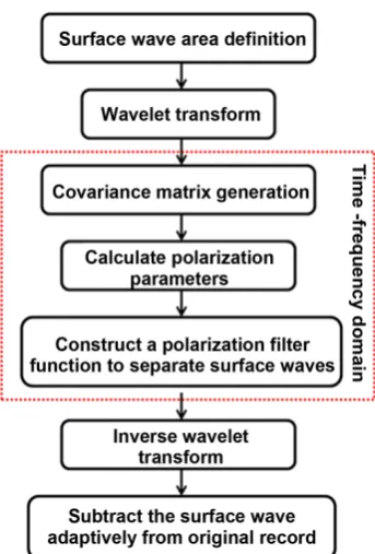
According to the polarization filtering principle and the actual data, the processing flow of the polarization filtering suppression surface wave is summa-rized in Figure 1.

The specific steps of polarization filtering are as follows: 1) Define the surface wave suppression window

Since the propagation characteristics of surface waves are only related to the geological features of the surface, the surface wave velocity of the same area are almost consistent. On a single shot record, the surface waves are fan-shaped. According to this feature of the surface wave, the window area for suppressing surface waves can be defined as follow:

( )

0 x

t x t

v

= + (20)

where t(x) is the start time of the surface wave suppression; x is the offset; t0 is the start time of the time window; v is the apparent velocity of the surface wave.

2) Wavelet transform, convert the seismic data to the time-frequency domain. 3) Generate the covariance matrix of multi-component seismic trace.

4) Calculate the polarization characteristic parameters in the time-frequency domain.

5) Use polarization filtering to separate surface wave. The body wave propa-gating in a homogeneous isotropic medium is a linearly polarized wave, and the surface wave is an elliptical polarized wave. However, in the case of anisotropic medium or interference, the particle vibration of the wave becomes very com-plicated. The wave often appears as an irregular ellipse with a large flattening rate. Therefore, in the polarization filtering, the polarization filtering parameters should be reasonably set according to the characteristics of the actual data.

6) Inverse wavelet transform, convert the surface wave energy to the time do-main.

7) Subtract the surface wave from the original record adaptively.

(7)

[image:7.595.286.458.66.320.2]

Figure 1. The flowchart of polarization filtering.

from raw converted wave in the time-frequency domain, then the surface wave was subtracted from the raw record adaptively in the time domain.

4. Examples

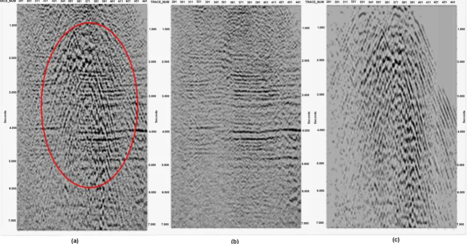
Figure 2(a) is a shot record of converted wave acquired in a certain area of Sau-di Arabia. The surface wave has a wide spatial Sau-distribution and strong energy in the original single shot, which seriously pollutes the effective signal. Figure 2 and Figure 3 show the single shot and stack profiles before and after applying the polarization filtering proposed in this paper. Before the noise is suppressed, the event on the stack profile is covered by the surface wave energy. It is difficult to identify a continuous event, which has a great impact on subsequent processing. After the polarization filtering, as shown as Figure 2(b) and Figure 3(b), both the shot and stack profiles have clear events, and the signal-to-noise ratio is greatly improved. As we can see from Figure 2(c) and Figure 3(c), the noise suppressed, the polarization filtering does not damage the effective reflec-tion energy.

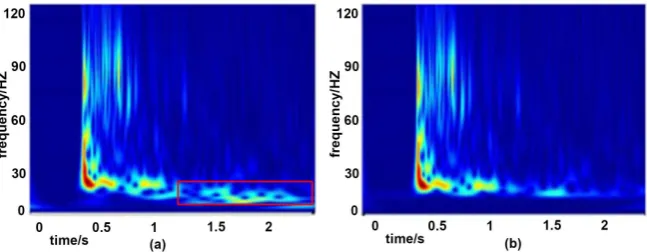
Figure 4 shows the time-frequency spectrum before and after the surface wave attenuation. Before the surface wave is suppressed, there is noise energy between 0 - 15 Hz in the low frequency band. After the surface wave is attenuated, the noise energy of the frequency band is greatly reduced.

5. Conclusions

(8)

[image:8.595.63.538.73.315.2]

Figure 2. The single shot comparison before and after polarization filtering (a) shot gather before polarization filtering; (b) shot gather after polarization filtering; (c) and the surface wave removed.

Figure 3. The stack section comparison before and after polarization filtering (a) stack section before polarization filtering; (b) stack section after polarization filtering; (c) the surface wave removed.

[image:8.595.61.537.366.614.2]

(9)

[image:9.595.213.537.74.200.2]

Figure 4. Comparison of spectrum between before and after polarization filtering: (a) the spectrum before surface wave attenuation; (b) the spectrum after surface wave attenua-tion.

By transforming the separated surface wave from time-frequency domain to the time domain, and then subtracting the surface wave from the raw record in time domain adaptively, this processing make the denoising effect more natural.

Conflicts of Interest

The authors declare no conflicts of interest regarding the publication of this pa-per.

References

[1] Shimshoni, M. and Smith, S.W. (1964) Seismic Signal Enhancement with Three-Component Detectors. Geophysics, 29, 664-671.

https://doi.org/10.1190/1.1439402

[2] Flinn, E.A. (1965) Signal Analysis Using Rectilinearity and Direction of Particle Motion. Proceedings of the IEEE, 53, 1874-1876.

https://doi.org/10.1109/PROC.1965.4462

[3] Samson, J.C. (1977) Matrix and Stokes Vector Representation of Detectors for Pola-rized Wave-Forms. Geophysical Journal of the Royal Astronomical Society, 51, 583-603.https://doi.org/10.1111/j.1365-246X.1977.tb04208.x

[4] Benhama, A., Cliet, C. and Dubesset, M. (1988) Study and Application of Spatial Directional Filtering in Three-Component Recordings. Geophysical Prospecting, 36, 591-613.https://doi.org/10.1111/j.1365-2478.1988.tb02182.x

[5] Jurkevics, A. (1988) Polarization Analysis of Three-Component Array Data. Bulle-tin of the Seismological Society of America, 78, 1725-1743.

[6] Shieh, C. and Herrmann, R.B. (1990) Ground Roll: Rejection Using Polarization Filters. Geophysics, 55, 1216-1222.https://doi.org/10.1190/1.1442937

[7] Huang, Z.Y., Gao, L., Xu, Y.M., et al. (1996) The Analysis of Polarization in Three-Component Seismic Data and Its Application. Geophysical Prospecting for Petroleum, 35, 9-16.

[8] Chen, Y., Zhang, Z.J. and Tian, X.B. (2005) Complex Polarization Analysis Based on Windowed Hilbert Transform and Its Application. Geophysics, 48, 889-895.

https://doi.org/10.1002/cjg2.736

(10)

DOI: 10.4236/ijg.2019.104028 490 International Journal of Geosciences [10] Christoffersson, A., Husebye, E.S. and Ingate, S.F. (1985) A New Technique for

3-Component Seismogram Analysis. Semiannual Technical Summary, 2, 85-86. [11] Jackson, G.M., Mason, I.M. and Greenhalgh, S.A. (1991) Principal Component

Transforms of Triaxial Recordings by Singular Value Decomposition. Geophysics, 56, 528-533.https://doi.org/10.1190/1.1443068

[12] Vidale, T. (1986) Complex Polarization Analysis of Particle Motion. Bulletin of the Seismological Society of America, 76, 1393-1405.

[13] Rene, R.M., Fitter, J.L., Forsyth, P.M., et al. (1986) Multi-Component Seismic Stu-dies Using Complex Trace Analysis. Geophysics, 51, 1235-1251.

https://doi.org/10.1190/1.1442177

[14] Stewart, R.R. (1990) Ground-Roll Filtering Using Local Instantaneous Polarization. Crewes, 97, 28-33.

[15] Morozov, L.B. and Smithson, S.B. (1996) Instantaneous Polarization Attributes and Directional Filtering. Geophysics, 61, 872-881.https://doi.org/10.1190/1.1444012 [16] Zhang, Y. and Zhou, J. (1999) Analysis of Factors Affecting Spatial Direction

Fil-tering Effect. Oil and Gas Geology, 20, 212-215.

[17] Tatham, R.H. and McCormack, M.D. (1991) Multicomponent Seismology in Petro-leum Exploration. Society of Exploration Geophysicists.