Existence of Periodic Solution for a Non Autonomous Stage Structured Predator Prey System with Impulsive Effects

(1)

Applied Mathematics, 2011, 2, 355-362

doi:10.4236/am.2011.23042 Published Online March 2011 (http://www.SciRP.org/journal/am)

Existence of Periodic Solution for a Non-Autonomous

Stage-Structured Predator-Prey System with Impulsive

Effects

Lifeng Wu, Zuoliang Xiong, Yiping Deng

Department of Mathematics, Nanchang University, Nanchang, China E-mail: [email protected]

Received November 20, 2010; revised January 25, 2011; accepted January 28, 2011

Abstract

In this paper, we studied a non-autonomous predator-prey system where the prey dispersal in a two-patch environment. With the help of a continuation theorem based on coincidence degree theory, we establish suf-ficient conditions for the existence of positive periodic solutions. Finally, we give numerical analysis to show the effectiveness of our theoretical results.

Keywords:Periodic Solution, Coincidence Degree Theory, Stage-Structured, Impulsive

1. Introduction

In recent years, non-autonomous predator-prey systems have been widely studied [1-6]. There has been a grow-ing interest in the study of mathematical models of pop-ulations dispersing among patches in the nature world [3,7-9].

In the classical predator-prey models it is usually as-sumed that each individual predator admits the same abi- lity to feed on prey. However, it is different for some species whose individuals have a life history that takes them through two stages, immature and mature, where immature predators are raised by their parents, so many models with time delays and stage structure for both prey and predator were investigated and rich dynamics have been observed [4,6,10-12].

In this paper, we are considered the effects of prey diffusion in two patches and maturation delay for predator on the dynamics of an impulsive predator-prey model. We discuss the differential equation: (See 1.1)

Where we suppose that the system is composed of two patches connected by diffusion. x t1

 

and x t2

 

represent the densities of prey species in patch I and II at time t,

 

1

y t and y2

 

t represent the densities of the imma-

ture and mature predator at time t in patch II, respectively.

 

1 ,

x t x₂

 

t can diffuse between patch I and II while the predator species is confined to patch II.  repre- sents a constant time to maturity. a t ii

 

1, 2



is the intrinsic

 

       





   



 



 

   



   



     

   



 



       







 



   

  





 



   

 

1 1 1 1 1

1 2 1

2 2 2 2 2

2 2

2 1 2

1 2 2

( )

2 2

2 1 1 1

( )

2 2 2

1 1

,

1

t t

k

r s ds

k

x t x t a t r t x t

d t x t x t

x t x t a t r t x t

k t x t y t

d t x t x t

t t

y t c t x t y t

c t e x t y t

d t y t q t y t

y t c t e x t y t

q t y t

x t



  

 









 

 

 



  



 _



  _

 

 _



   _{ }



  _



   _{ }



 _

 





  

 



  

 



  

 

1

2 2 2

1 1 2 2

,

1 , ,

k k

k k k k

k k k k k

x t

x t x t t t

y t y t y t y t

 



 

                  

 _

 _



 _{ } _

 

 

   

 _



(1.1)

growth rate;

 

  

1, 2



i i

r t i

a t 

is the carrying capacity;

 

1, 2



i

d t i is the dispersal rate of prey species;

 

(2)

competition. ik and krepresent the annual birth pul-

se of x ti

   

,y t1 i1, 2



at tk



k Z





 . We make the following assumptions for our model:

1)a ti

       

,r ti ,d ti ,q ti i1, 2 ,

      

d t ,k t ,c t and

 

r t are continuous positive periodic functions； 2) 1k, 2k and k are constants and there exists a po-

sitive integerqsuch that

1k q 1k, 2k q 2k, k q k,tk q tk

           .

2. Preliminaries

Denote byPC J R



,



JR



the set of functions :

JR, which are piecewise continuous in

 

0, , and have points of discontinuity t_k

 

0, . Let PC J R1



,



denote the set of functions  with derivative 

 

t 



,



PC J R . We define the Banach space of  periodic functions PC 



PC



 

0, ,R





 

0  

 



with

 

 





sup : 0,

PC t t

     and 1

PC_ with _PC1



 



1



max ( ) ,

PC PC

t

 

  , we will considered the PCPCwith the norm

1 2

( , )

PC

   ₁ ₂

PC PC

  .

We define:

 

0

1

f  f t dt 



_

,

 

[0, ]

min

L

t

f f t

 

 ,

 

[0, ]

max

M

t

f f t

 

 .

3. Existence of Positive Periodic Solutions

In this section, we study the existence of positive period-ic solutions of system (1.1).

Before stating our result on positive periodic solu-tions of system (1.1), we need the following lemma: Lemma 3.1 ([13]). Let Xbe an open bounded set. Let L be a Fredholm mapping of index zero and N

be Lcompact on . Assume

1)for each

 

0,1 ,

x

is any solution ofLxNx

such thatx ;

2)for eachQNx0for eachx  KerL; 3) deg



JQN, KerL, 0



0.

Then the equation LxNx has at least one solution in  DomL.

Theorem 3.1If the system (1.1) satisfies

(H1)





1

ln 1 0

q

k k

a 



 

 _  _





 ,





1

ln 1 0

q

k k

d 



 

 _  _





 ,

(H2) 1 1





1

ln 1 0

q

k k

a d 



 

  _  _





 ,





4

2 2 2

1

ln 1 0

q M

M

k k

a d k e  



 

   _  _





 ,

(H3) _{c e}L m2m4 _{c e}M rLM2M4 ₀_,

then the system (1.1) has at least one periodic posi-tive solution.

Proof. Let

 

1 

 

2 

 

3 

1 , 2 , 1 ,

u t u t u t

x t e x t e y t e

 

4 

2

u t

y t e , then

 

   

 

_{ }

   

 

_{ }

 

   

_{ }

   

     

_{ }

 





       

  



       

 

1 2 1

2 4

1 2

2 4 3 3

2 4 3

2 4 4

4

1 1 1 1

1

2 2 2

2 2

3 1

4

2 ,

,

t t t t

u t u t u t

u t u t

u t u t

u t u t u t u t

r s ds u t u t u t

u t

u t a t r t e d t e

d t

u t a t r t e k t e

d t e d t

t

u t c t e d t q t e

c t e e

u t c t e e

q t e



 



 

    





  



 



   



  _

 

   _



  _



  



 _



,

k

t

              

 





 





 





 

1 1 1

2 2 2

3 3 4 4

ln 1 ,

ln 1 , ,

k k k

k k k k

k k k k k

u t u t

u t u t t t

u t u t u t u t

  



 

    

 

 _ _ _  _

 

 

   

 _



(3.1) One can easily see that if system (3.1) has one  periodic solution



1

       

, 2 , 3 , 4



T

u t u t u t u t , then

       



1 2 3 4





       



1 2 1 2

, , , T , , , T

u t u t u t u t

e e e e  x t x t y t y t

is a positive periodic solution of system(1.1). Thus, in what follows our goal is to show that system (3.1) has at least one periodic solution.

Here, we rewrite

 

   

 

1 1 , 2 2 ,

f t u t f t u t

 

   

 

3 3 , 4 4

f t u t f t u t . Let

1 1 1

DomLPC_PC_PC_

and

1 1 1

:

(3)

 













1 1 1 2 2 2 3 3

4 4 1

ln 1 ln 1 , ln 1 0 q k k k k f t u f t u N

u f t

u _f _t

         __ _    _   __  _  _             _ _ _ _ _        _{ } _    __ _ _ and

 

1 1 1

2 2 2 4

3 3 3

4 4 4

: , 0,

u u C

KerL R t

u u C

               _{    } _  __{    } _  _ _{    } _        _{    } _    .

Where Q is defined by

 

0 1 0 1 0 1 1 0 1 0 0 1 , 0 0 q k k q q k k q k k k q k k

f t dt a g t dt b QZ

h t dt c j t dt d                      _{  }_{ }    _  __{ }_    _{ }_{ }_      _{ }    _  _{ }     __{ }_       _  _   _ _   

















.

Furthermore, KP: ImLKerPDomLis given by

 

0 0 0

0 1

0 0 0

0 1

0 0 0

0 1

0 0 0

0 1 1 1 1 1 k k k k q t k k

t t k

q t

k k

t t k

P _q

t

k k

t t k

q t

k k

t t k

f t dt a f s dsdt a

g t dt b g s dsdt b

K Z

h t dt c h s dsdt c

j t dt d j s dsdt d

                         _ _ _                   _ _ _       _ _ _     





 





 





 





 

. Thus,





 





 





 





 

1 1 0 0 1 2 2 0 2 0 3 3 1 0 0 4 4 0 ln 1 ln 1 ln 1 k k k k t t k t t P k t t

f t dt

u

f t dt u

K I Q N

u

f t dt u

f t dt

              _ _                   _{ }_{ } _             _ _    













 





 





 





 

1 1 0 0 1 2 2 0 0 1 3 0 0 1 4 0 0 1 ln 1 1 ln 1 1 ln 1 1 q t k k q t k k q t k k t f s dsdt

f s dsdt

                                            



 



 



 

 





 





 





 

1 1 0 1 2 2 0 1 3 0 1 4 0 1 1 ln 1 2 1 1 ln 1 2 1 1 ln 1 2 1 1 2 q t k k q t k k q t k k t

f s dt t

f s dt t

f s dt t        _  _ _  _ _    _ _            _ _  _  _         _ _   _  _   _ _   













In order to apply the Lemma 3.1, we also need to find an appropriate open and bounded subset . Corrspon-ing to the operator equation LuNu, here, 

 

0,1 ,



1, 2, 3, 4



T

u u u u u , we can get

 

   

 

   

 





 





 





 

1 1 2 2

3 3 4 4

1 1 1

2 2 2

3 3

4 4

, ,

,

, ,

ln 1 , ln 1 ,

, ln 1 , ,

k

k k k

k

k k k

k k

u t f t u t f t t t u t f t u t f t u t u t

u t u t

t t u t u t

u t u t

                 _       _         _ _ _ _  _{ }             _      (3.2)

Suppose



1, 2, 3, 4



T

u u u u u is a periodic solution to (3.2). By integrating over

 

0, ,





 

   









 

_{ }

 

_{ }

   









 

     

_{ }

 









      2 1 1

2 4 1 2

2 4 3 3

2 4

1 1 1

1

( )

1 1

0

2 2 2

1 2 2 0 1 1 0 1 ln 1 1 , 1 ln 1 1 , 1 ln 1 1 1 t t q k k

u t u t u t

q k k

u t u t u t u t

q k k

u t u t u t u t

r s ds u t u t u

a d

r t e d t e dt

a d

r t e k t e d t e dt

d

c t e q t e dt

c t e  e

                                  _  _         _  _         _  _      













 





        3 4

2 4 4

0 ( ) 2 0 0 , 1 1 , t t t u t

r s ds u t u t u t

dt

q t e dt

c t e  e dt

(4)

 

_{ }

   





1 2 1

1 1 1

0 0

1 1

0

1 1 1

1

2 ln 1

u t u t u t

q

k k

u t dt a t d t dt r t e d t e dt a d

 



 





 

 

 

   _  _

 







(3.4)

 





2 2 2 2

0

1

2 ln 1

q

k k

u t dt a d 

 



 

   _  _









 (3.5)

 





3 0

1

2 ln 1

q

k k

u t dt d 

 



 

  _  _









 (3.6)

 

4 

4 2

0 20

u t

u t dt q t e dt

 









(3.7) Scinceu ti

 

PC , i, i

 

0,



i1, 2, 3, 4



, such that

 

_{ }

   

_{ }

 

0, 0,

min , max

i i i i i i

t t

u u t u u t

 

 

 

  .

Letv t

 

max



u t u1

   

, 2 t



, then v t

 

PC

1) ifu t1

 

u2

 

t oru t1

 

u2

 

t , butu t1

 

u2

 

t ,

thenv t

 

u t1

 

and

 



   

1 





1 



1 1 1 1 1

u t M L u t

u t  a t r t e  a r e ; 2) ifu2

 

t u t1

 

oru t1

 

u2

 

t , butu2

 

t u t1

 

,

thenv t

 

u2

 

t and

 



 

2 





2 



2 2 2 2 2

u t M L u t

u t  a t r t e  a r e . Dnote



1 2





1 2



max M, M , min L, L ,

a a a p r r k max



 1k, 2k



,

then

 



 



 





, ,

ln 1 , ,

v t

k

k k k

D v t a pe t t

v t t t



 



 _ _ _

 

   

 (3.8)

Integrating (3.8) over

 

0, , we get





 

0 1

ln 1

q

v t k

k

a p e dt

 



 

 _  _ 









.

Therefore,

    1





0 0

ln 1

i i i

q

k k

u u t

a

e dt e dt

p

  

 



 

 _  _

 

 





(3.9)

 

1









ln 1

ln 1, 2

q

k k

i i

a

u i

p

 







 

 _  _

 





 ,

 

















0

1

ln 1

ln

2 ln 1 1, 2 ,

q

i i i i ik

k q

k k

q

i i ik i

k

u t u u t dt

a

p

a d M i



 

 



 



 

   _  _

 

 

 _  _

 



 _ _

 _   _  __ 

 

 









(3.10)

According to the fourth equation of (3.3), we have

 

24 

_

_

  2  4 

2

0 0 ,

t t r s ds

u t u t u t

q t e dt c t e  e dt

  _ _

    

 



(3.11)

   

 

4 2 4

4 2

2

2 ₀ ₀

0 ,

L L

u t r M u t

L M

u t

r M

M

q e dt c e dt

c e e dt

  _ _

 

   

 

 



(3.12)

Due to



4



4 

2

2 ( )

0 0

u t u t

e dt e dt

 







(3.13) From (3.11) and (3.12), we have

 

4 2

0

2

L

u t M r M

L

e dt c e

q

  _ __





(3.14)

 

2

4 4

2

ln

L

r M

M

L c e u

q



   

According to (3.7) and (3.14), we get

 

4

2 4

4 2

0 0

2 2 ₀

2

2 2

2 ,

L

u t

r M

M M

u t M

L

u t dt q t e dt q c e q e dt

q

 



   



 





 

2 2

4 4 4 ₀ 4 2

4

2 2

2

ln ,

L L _M _M _r _M

r M

M

L L

u t u u t dt

q c e c e

M

q q



 



  

 

 

  





(3.15)

According to the third equation of (3.3), we have

 

2  4  3 

_

_

0

1

ln 1

q u t u t u t

k k

c t e dt d



 

 



 

  _  _









,

Duo tou2

 

t M u2, 4

 

t M4, we have

 

_

_

3 2 4

0

1

ln 1

q u t

M M

M

k k

c e  e dt d  

 

  _  _









,

 





2 4 3 3

1

ln

ln 1

M M

M

q

k k

c e u

d

 

 







 

 _  _







,

(5)

 













2 4 3 3 3 ₀ 3

1 1 3 1 ln 1 ln ln 1

2 ln 1 ,

q k k M M M q k k q k k

u t u u t dt

c e d d M                  _  _       _  _    _ _  _  _  __    







 (3.16)

From the first equation of (3.3), we have

 

_{ }

 





1 1 1

1 1 1 1

0 0

1 1

ln 1 ,

u u t

q k k

r t e dt r t e dt a d

 _           _  _  





So,

 

1 1 1



1



1 1 1 ln 1 ln q k k a d u r          _  _   



,

 













1 1 1 ₀ 1 1

1

1 1 1

1

1 1 1 1

1

ln 1

ln

2 ln 1 ,

q k k q k k q k k

u t u u t dt

a d

r

a d m

                _  _       _  _     _ _  _   _  __    







 (3.17)

From the second equation of (3.3), we have

 

2 

_

_

4

2 2 2 2

0 1 ln 1 , q u t k k M M

r t e dt a d k e           _  _   





 





4

2 2 2

1 2 2 2 ln 1 ln , q M M k k

a d k e

u r           _  _   



4

2 2 2 ₀ 2 2

1

2 2 2

1 2

2 2 2 2

1

( ) ( ) ( ) ln[ (1 )]

ln[ (1 )]

ln

2 ln[ (1 )] ,

q k k q M M k k q k k

u t u u t dt

a d k e

r

a d m

                        _    _  







 (3.18) From (3.11) we have

4 4 4 4

2 4

( ) ( ) 2 ( )

2 ₀ ₀ 2

( ) 0 ( )

,

M

u u t u t

M

r m u t

L

q e e dt q t e dt

c e e dt

        



 

2

4 4 2 ln M r m L M c e u q      ,

 

4 

2 2

4 4 4 2 ₀ 2 4 2 2 2 2 ln , L M u t M r M M M r m L M L

u t u q e dt

q c e c e m q q              



(3.19)

According to the third equation of (3.3), we have





 





3

2 4 2 4

3

0 1

1

ln 1 ,

L _u _t

m m r M M

L M q M M k k

c e c e e dt

d q e

                _  _  





Similarly, we have

 





2 4 2 4

3 3 3 1 1 ln ln 1 L

m m r M M

L M q M M k k

c e c e

u

d q e

               _  _ 



 ,

 













2 4 2 4

3

3 3 3 ₀ 3

1 1 1 3 1 ln 1 ln ln 1

2 ln 1 ,

L

q k k

m m r M M

L M q M M k k q k k

u t u u t dt

c e c e

d q e

d m                     _  _         _  _       _  _  __    







 (3.20)

Thus, we have

 









1 2 3 4 1 2 3 4

(0, )

sup max , , , , , , ,

1, 2, 3, 4 ,

i t

i

u t M M M M m m m m

D i



 

 

Denote M max



D D D D1, 2, 3, 4



D0 ,where D0may

be taken sufficiently large such that each solution to Eq-uations (3.21)













       









       

1 2 1

2 4 1 2

2 4 3

3

2 4 3 4

1 1 1 1 1

1

2 2 2 2 2

1

2 1

ln 1 ,

1

ln 1 ,

1

ln 1 ,

, t t t t q

u u u

k k

q

u u u u

k k

r s ds u t u t u t u u u

q u

k k

r s ds u t u t u t u

a d r e d e

a d r e ke d e

ce c t e e

d q e

c t e e q e

(6)

satisfies



1, 2, 3, 4



0

T

u u u u    D , then u M. Denote:DomL

 

0,1 X as the form





















       

1

2

3

2 4 3 4

1 2 3 4

1 1 1 1

1

2 2 2 2

1 1

1

2

, , , ,

1

ln 1

1

ln 1

1

ln 1

t t

q u

k k

q u

k k

q u

k k

u u u u

a d r e

d q e

c t e  e   q e

 

 

 

 



    





   

   

   

 

 

 _ _ 

 _ _ _ _ _ _ 

 _ _ 

 

 

 _{ } _ _ 

 

 _ _ 

 

 _ _ 

 







       

2 1

4 1 2

2 4 3

1

2

,

0

t t

u u

u u u

r s ds u t u t u t u u u

d e

ke d e

ce c t e  e  



 



    

  

 

 

 

 

  

   

 

 

Where

 

0,1 is a parameter. With the mapping, we have 



u u u u1, 2, 3, 4,



0 for



1, 2, 3, 4



T

u u u u 

KerL

  . So we know that u M .

Obviously, the algebraic Equation (3.22) has a unique solution



u u u u1, 2, 3, 4



   

.

















       

1

2

3

2 4 3 4

1 1 1 1

1

2 2 2 2

1 1

1

2

1

ln 1 0,

1

ln 1 0,

1

ln 1 0,

0,

t t

q u

k k

q u

k k

q u

k k

a d r e

d q e

c t e  e   q e

 

 

 



    



  

    

  

 



 _ _

    _  _

 _ _



 _ _

   _  _

  



   





(3.22)

From the coincidence degree theory, we can obtain







1 2 3 4



deg , , 0

deg ( , , , , ), , 0 1.

JQNu KerL

u u u u KerL

 

 

   

4. Numerical Analysis

In this paper, we have focused on the dynamics comple- xity of a stage-structured system with diffusion and im-pulsive effects. By using the method of coincidence de-gree, we obtain the sufficient condition for the existence of at least one positive  periodic solution. In this section, we give the numerical results.

 

   

 

     

   

 



 



   











 



 



 



 

1 1 1

2 1

2 2 2

2 2

1 2

1 2 2

0.8

2 2

2

1 1

2

[3 1.6cos t 1.5 ]

(2 cos t [ ],

[5.2 3.2 sin 2.4 ]

(3 2.5sin )

(2 1.2 sin )[ ],

1.2 sin

1.2 sin(

0.2 1 0.5 cos ,

1 0.75

x t x t x t

x t x t

x t x t t x t

t x t y t

t x t x t

y t t x t y t

t e x t y t

y t t y t

y t

 

   

 

  

  

  

 

  

  

   

  

  





 



 











 



 



  

 



  

 





 

2 2 0.8

2 2

1 1 1

2 2 2

1 1 2 2

,

cos

(1.2 sin ,

1 ,

1 , ,

k

k k

k k k

k k k k

t t

t y t

t e x t y t

x t x t

x t x t t t

y t y t y t y t



   

  





 

 

 



 _ _

 _



 

 



 



   

 _



   



 _

   _ 

 _

 _{ } _ _



(4.1)

Numerical analysis indicates that the complex dynam-ic behavior of system (1.1) depends on the values of im-pulsive perturbationsk,ik



i1, 2



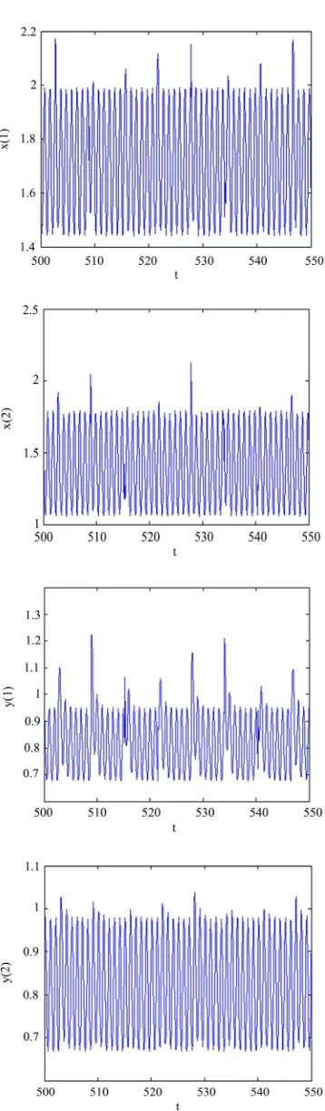
in model (1.1). Our

theoretical results are confirmed by numerical simula-tions. we can see that the dynamic behavior of the system (4.1) has obviously varied as the impulse value changing. Let10.001,20.002,0.003, it is easily proved

that the system (4.1) satisfies all the conditions of Theo-rem 3.1, that mean the system (4.1) has at least one posi-tive periodic solution (Figure 1). As impulses increase, the periodic oscillation of system (4.1) will be destroyed (Figure 2).

5. Acknowledgments

This work is supported by Natural Science Foundation of Jiangxi Province. (No. 2009GZS0020)

6. Conclusions

(7)

[image:7.595.335.514.66.678.2]

Figure 1. Dynamic behavior of the system (4.1) with initial values



1.2,1.2,0.8,0.6



,τ= 0.1and impulsive perturbations

1= 0.001

[image:7.595.81.259.75.669.2]

θ ,θ₂= 0.002,φ= 0.003.

Figure 2. Dynamic behavior of the system (4.1) with initial values



1.2,1.2,0.8,0.6



,τ= 0.1and impulsive perturbations

1= 0.1

(8)

leave these aspects for future research.

7. References

[1] Y. Nakata, Y. Muroya, “Permanence for Nonautonomous Lotka-Volterra Cooperative Systems with Delays,” Non-linear Anal, Vol. 11, No. 1, 2010, pp. 528-534.

doi:10.1016/j.nonrwa.2009.01.002

[2] T. V. Ton, “Survival of Three Species in a Nonautonom-ous Lotka-Volterra System,” Journal of Mathematical

Analysis and Applications, Vol. 362, No. 2, February

2010, pp. 427-437. doi:10.1016/j.jmaa.2009.07.053 [3] S. H. Chen, J. H. Zhang and T. Young, “Existence of

Positive Periodic Solution for Nonautonomous Preda-tor-Prey System with Diffusion and Time Delay,” Jour-nal of ComputatioJour-nal and Applied Mathematics, Vol. 159, No. 2, October 2003, pp. 375-386.

doi:10.1016/S0377-0427(03)00540-5

[4] Z. H. Lu, X. B. Chi and L. S. Chen, “Global Attractivity of Nonautonomous Stage-Structured Population Models with Dispersal and Harvest,” Journal of Computational

and Applied Mathematics, Vol. 166, No. 2, April 2004,

pp. 411-425. doi:10.1016/j.cam.2003.08.040

[5] Z. D. Teng and L. S. Chen, “Uniform Persistence and Existence of Strictly Positive Solutions in Nonautonom-ous Lotka-Volterra Competitive Systems with Delays,”

Computers & Mathematics with Applications, Vol. 37, No. 7, April 1999, pp. 61-71.

doi:10.1016/S0898-1221(99)00087-5

[6] J. Y. Wang, Q. S. Lu and Z. S. Feng, “A Nonautonomous Predator-Prey System with Stage Structure and Double Time Delays,” Journal of Computational and Applied

Mathematics, Vol. 230, No. 1, August 2009, pp. 283-299. doi:10.1016/j.cam.2008.11.014

[7] X. X. Liu and L. H. Huang, “Permanence and Periodic Solutions for a Diffusive Ratio-Dependent Predator-Prey System,” Applied Mathematical Modelling, Vol. 33, February 2009, pp. 683-691.

doi:10.1016/j.apm.2007.12.002

[8] Z. X. Hu, G. K. Gao and W. B. Ma, “Dynamics of a Three-Species Ratio-Dependent Diffusive Model,” Non-linear Anal, Vol. 217, November 2010, pp. 1825-1830. [9] C. J. Xu, X. H. Tang and M. X. Liao, “Stability and

Bbi-furcation Analysis of a Delayed Predator-Prey Model of Prey Dispersal in Two-Patch Environments,” Applied

Mathematics and Computation, Vol. 216, July 2010, pp.

2920-2936. doi:10.1016/j.amc.2010.04.004

[10] S. Q. Liu, L. S. Chen and Z. J. Liu, “Extinction and Per-manence in Nonautonomous Competitive System with Stage Structure,” Journal of Mathematical Analysis and Applications,Vol. 274, No. 2, October 2002, pp. 667-684. doi:10.1016/S0022-247X(02)00329-3

[11] Z. Li and F. D. Chen, “Extinction in Periodic Competitive Stage-Structured Lotka-Volterra Model with the Effects of Toxic Substances,” Journal of Computational and Ap-plied Mathematics, Vol. 231, No. 1, September 2009, pp. 143-153. doi:10.1016/j.cam.2009.02.004

[12] X. W. Jiang, Q. Song and M. Y. Hao, “Dynamics Beha-viors of a Delayed Stage-Structured Predator-Prey Model with Impulsive Effect,” Applied Mathematics and Com-putation, Vol. 215, No. 12, February 2010, pp. 4221-4229. doi:10.1016/j.amc.2009.12.044