THE SLOAN DIGITAL SKY SURVEY REVERBERATION MAPPING PROJECT: FIRST BROAD-LINE H
β
AND
Mg
IILAGS AT
z
0.3 FROM SIX-MONTH SPECTROSCOPY
Yue Shen1,2,25, Keith Horne3, C. J. Grier4,5, Bradley M. Peterson6,7, Kelly D. Denney6,7,26, Jonathan R. Trump4,5,25, Mouyuan Sun4,5,8, W. N. Brandt4,5,9, Christopher S. Kochanek6,7, Kyle S. Dawson10, Paul J. Green11, Jenny E. Greene12, Patrick B. Hall13, Luis C. Ho14,15, Linhua Jiang14, Karen Kinemuchi16, Ian D. McGreer17, Patrick Petitjean18, Gordon T. Richards19, Donald P. Schneider4,5, Michael A. Strauss12, Charling Tao20,21, W. M. Wood-Vasey22, Ying Zu23, Kaike Pan16, Dmitry Bizyaev16, Jian Ge24, Daniel Oravetz16, and Audrey Simmons16
1
Department of Astronomy and National Center for Supercomputing Applications, University of Illinois at Urbana-Champaign, Urbana, IL 61801, USA
2
Carnegie Observatories, 813 Santa Barbara Street, Pasadena, CA 91101, USA
3
SUPA Physics/Astronomy, Univ. of St. Andrews, St. Andrews KY16 9SS, Scotland, UK
4
Department of Astronomy & Astrophysics, The Pennsylvania State University, University Park, PA, 16802, USA
5
Institute for Gravitation and the Cosmos, The Pennsylvania State University, University Park, PA 16802, USA
6
Department of Astronomy, The Ohio State University, 140 West 18th Avenue, Columbus, OH 43210, USA
7
Center for Cosmology and AstroParticle Physics, The Ohio State University, 191 West Woodruff Avenue, Columbus, OH 43210, USA
8
Department of Astronomy and Institute of Theoretical Physics and Astrophysics, Xiamen University, Xiamen, Fujian 361005, China
9
Department of Physics, 104 Davey Lab, The Pennsylvania State University, University Park, PA 16802, USA
10Department of Physics and Astronomy, University of Utah, Salt Lake City, UT 84112, USA 11
Harvard-Smithsonian Center for Astrophysics, 60 Garden Street, Cambridge, MA 02138, USA
12
Department of Astrophysical Sciences, Princeton University, Princeton, NJ 08544, USA
13
Physics and Astronomy Department, York University, Toronto, Ontario M3J 1P3, Canada
14
Kavli Institute for Astronomy and Astrophysics, Peking University, Beijing 100871, China
15
Department of Astronomy, School of Physics, Peking University, Beijing 100871, China
16
Apache Point Observatory and New Mexico State University, P.O. Box 59, Sunspot, NM 88349-0059, USA
17
Steward Observatory, The University of Arizona, 933 North Cherry Avenue, Tucson, AZ 85721-0065, USA
18
Institut d’Astrophysique de Paris, Université Paris 6 and CNRS, 98bis Boulevard Arago, F-75014 Paris, France
19
Department of Physics, Drexel University, 3141 Chestnut Street, Philadelphia, PA 19104, USA
20
Centre de Physique des Particules de Marseille, Aix-Marseille Université, CNRS/IN2P3, 163, avenue de Luminy—Case 902—F-13288 Marseille Cedex 09, France
21
Tsinghua Center for Astrophysics, Tsinghua University, Beijing 100084, China
22
PITT PACC, Department of Physics and Astronomy, University of Pittsburgh, 3941 O’Hara Street, Pittsburgh, PA 15260, USA
23
McWilliams Center for Cosmology, Department of Physics, Carnegie Mellon University, 5000 Forbes Avenue, Pittsburgh, PA 15213, USA
24
Astronomy Department, University of Florida, 211 Bryant Space Science Center, Gainesville, FL 32611, USA Received 2015 October 9; accepted 2015 December 9; published 2016 February 4
ABSTRACT
Reverberation mapping(RM)measurements of broad-line region(BLR)lags inz>0.3quasars are important for directly measuring black hole masses in these distant objects, but so far there have been limited attempts and success given the practical difficulties of RM in this regime. Here we report preliminary results of 15 BLR lag measurements from the Sloan Digital Sky Survey Reverberation Mapping(SDSS-RM)project, a dedicated RM program with multi-object spectroscopy designed for RM over a wide redshift range. The lags are based on the 2014 spectroscopic light curves alone(32 epochs over six months)and focus on the Hβand MgIIbroad lines in the
100 lowest-redshift(z<0.8)quasars included in RM; they represent a small subset of the lags that SDSS-RM(including 849 quasars toz~4.5)is expected to deliver. The reported preliminary lag measurements are for intermediate-luminosity quasars at 0.3z<0.8, including nine Hβ lags and six MgII lags, for the first time
extending RM results to this redshift–luminosity regime and providing direct quasar black hole mass estimates over approximately half of cosmic time. The MgIIlags also increase the number of known MgIIlags by several
foldand start to explore the utility of MgII for RM at high redshift. The location of these new lags at higher
redshifts on the observed BLR size–luminosity relationship is statistically consistent with previous Hβ results at
<
z 0.3. However, an independent constraint on the relationship slope atz>0.3is not yet possible owing to the limitations in our current sample. Our results demonstrate the general feasibility and potential of multi-object RM forz>0.3quasars.
Key words:black hole physics –galaxies: active–line: profiles –quasars: general–surveys
Supporting material:machine-readable tables
1. INTRODUCTION
Measuring the masses of black holes in quasars and active galactic nuclei (AGNs)27 is of critical importance to many
fundamental problems in AGN physics and phenomenology, the growth of supermassive black holes (SMBHs), and the coevolution of galaxies and SMBHs. As the primary method to measure active SMBH masses, the reverberation mapping (RM) technique estimates the size of the broad-line region (BLR)by measuring the time lag between continuum variations and line responses (Blandford & McKee 1982; Peter-son1993,2014). This technique has been widely practiced in The Astrophysical Journal,818:30(17pp), 2016 February 10 doi:10.3847/0004-637X/818/1/30
© 2016. The American Astronomical Society. All rights reserved.
25
Hubble Fellow.
26
NSF Astronomy & Astrophysics Postdoctoral Fellow.
27
We use the term “AGN” to refer to the low-luminosity counterparts of quasars.
the past two decades, resulting in BLR RM measurements for
∼60 low-redshift (z<0.3) AGNs and quasars(e.g., Peterson et al. 1998a, 2002, 2004; Kaspi et al. 2000, 2005; Bentz et al.2009,2010a,2013; Denney et al.2009,2010; Barth et al. 2011a,2011b,2013,2015; Rafter et al.2011,2013; Grier et al. 2012; Du et al.2014,2015; Hu et al.2015), mostly focused on the Hβline. Beyondz>0.3, however, RM results are scarce, given the stringent observational requirements for detecting lags in these distant and faint objects: there have been only a handful of attempts for the most luminous quasars(e.g., Kaspi et al. 2007; Trevese et al. 2007,2014), and only one or two tentative CIV/CIII]lag detections have been reported.
In addition to sample size and redshift coverage, another limitation of the current RM sample is the deficit of lag detections for the MgIIline, despite the fact that MgIIis one of
the most important lines of RM interest that can be observed in the optical at0.3< <z 2. Locally, there is only one reliable detection of an MgII lag in NGC 4151 (Metzroth
et al. 2006)and two marginal MgII lag detections in NGC
5548(Clavel et al.1991)and NGC 3783(Reichert et al.1994); all were based on UV spectroscopy from space. The prospects of MgIIRM in the optical for high-redshift quasars therefore
demand a systematic examination.
To expand the redshift range and AGN/quasar parameter space for RM measurements, and to evaluate the potential of RM on all prominent broad lines, we are conducting a dedicated multi-object RM program, Sloan Digital Sky Survey Reverberation Mapping (SDSS-RM). The first-year observa-tions were completed in 2014 as an ancillary program of the SDSS-III surveys (Eisenstein et al. 2011). SDSS-RM spectroscopically monitors a flux-limited (ipsf <21.7)sample of 849 quasars in a single 7 deg2 field with the SDSS-III
Baryon Oscillation Spectroscopic Survey(BOSS)spectrograph (Dawson et al. 2013; Smee et al. 2013) on the 2.5 m SDSS telescope (Gunn et al. 2006), accompanied by dedicated photometric monitoring from a number of ground-based wide-field imagers. With its multiplex advantage, SDSS-RM offers considerably higher efficiency than traditional RM programs executed in a serial modeand is designed to perform RM for a homogeneous selection of quasars over a wide redshift and luminosity range. The details of the program are described in Shen et al.(2015a).
In this work we report initial broad-line lag detections from the first-year SDSS-RM observations. These detections are based on the six-month spectroscopic data alone and demonstrate the feasibility of lag detections using only carefully calibrated multi-fiber spectroscopy. The reported detections are for Hβ and MgIIonlyand serve as a
proof-of-concept study of the general feasibility of multi-object RM programs; they do not represent the complete set of lag detections from SDSS-RM, nor do we quantify the complete-ness of lag detections and selection biases inherent to our program in this work. We also do not consider the important aspects of multiple line detections in the same object. More comprehensive analyses of the SDSS-RM data with different focuses are deferred to future work. Nevertheless, the lag detections reported here represent a significant advance in RM: (1)they form the largest sample of lag detections forz0.3 quasars, whose luminosities overlap with those in thez<0.3 RM sample but are much lower than those in the handful of
>
z 0.3 quasars previously monitored for RM, thus greatly expanding the luminosity–redshift range for which RM
observations have been successful; and(2)they constitutethe largest sample of MgII lag detections to date, starting to
explore the utility of this line for RM purposes.
We describe the data and technical details of the time series analysis in Section2and present our results in Section3. We conclude in Section4with a brief outline for future work. Aflat ΛCDM cosmology withW =L 0.7(W =0 0.3)and h0=0.7 is adopted throughout. By default the reported lags are in the quasar rest frame. For ease of discussion, we use “lowz” to refer toz<0.3.
2. DATA AND TIME SERIES ANALYSIS
The spectroscopic data were taken during seven dark/gray runs from 2014 January to Julyand consist of a total of 32 epochs with an average cadence of∼4 days; each epoch had a typical exposure time of 2 hr. The spectroscopic data were pipeline-processed as part of the SDSS-III Data Release 12 (Alam et al. 2015), followed by a custom flux calibration scheme and improved sky subtraction as described in Shen et al.(2015a). The improved spectrophotometry has a nominal accuracy of ~5%. The wavelength coverage of BOSS spectroscopy is ∼3650–10400 Å, with a spectral resolution of
~
R 2000. The typical signal-to-noise ratio (S/N) per 69
-km s 1 pixel averaged over the g band in a 2 hr exposure is ∼4.5 atgpsf=21.2.
Next, we perform a spectral refining procedure on the customflux-calibrated multi-epoch spectra, called“PrepSpec,” to reduce further the scatter in theflux calibration. As briefly described in Section 3.4 of Shen et al. (2015a), PrepSpec rescales theflux levels of each individual epoch by optimizing modelfits(in parameterized functional forms) to describe the continuum and broad-line variability patterns as functions of time and wavelength, using the fluxes of the narrow emission lines (in particular [OIII]λλ4959, 5007) as an internal
calibrator (e.g., van Groningen & Wanders 1992), which are assumed to remain constant over the relatively short monitoring period(e.g., Peterson et al.2013). This procedure improves the calibration of the relative spectrophotometry to2%for low-redshift quasars with strong narrow emission lines. Given the typical ~10% variability amplitude of the continuum and responding broad-line fluxes (e.g., Peterson 2014), this additional improvement of the spectrophotometry is essential for detecting BLR lags based on spectroscopy alone. As a by-product of PrepSpec, we obtained model light curves(LCs)for the desired broad emission line and continuumfluxes, as well as model mean and rms profiles of the broad lines. We use the rest-frame 5100 Å continuumflux as thefiducial continuum LC used in the time series analysis, given the proximity of this continuum to the narrow [OIII]λλ4959, 5007 lines that are
used to calibrate the spectrophotometry. Since thefitting was performed over a large number of pixels, the measurement uncertainties in the model fluxes are typically much smaller than the uncertainties offluxes directly measured over a narrow range of pixels, as reported in most previous RM work. These PrepSpec outputs form the basis for our following analysis.
We now describe PrepSpec in further detail.
2.1. PrepSpec Analysis
residual calibration errors. For each SDSS-RM spectrum in any given epoch, our PrepSpec model is
m l( ,t)=p t A( )[ ( )l +B(l,t)+C(l,t)]. ( )1
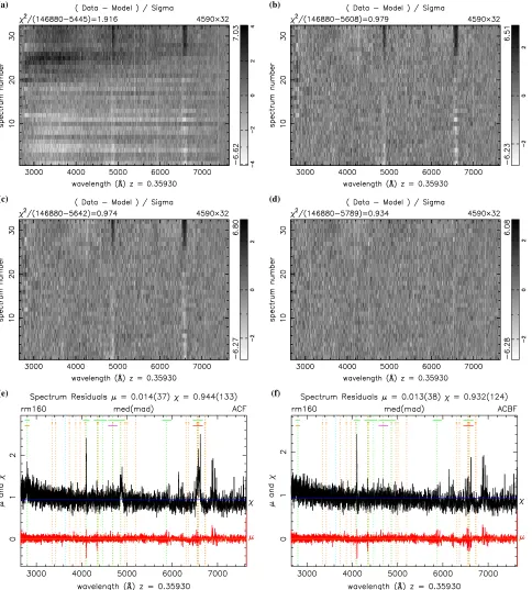
Herep(t)are time-dependent photometric corrections, A( )l is the average spectrum, andB(l,t)andC(l,t)are variations in the BLR spectrum and continuum, respectively. Corrections for residual wavelength shifts and spectral blurring were investi-gated and found not to be needed. Figures 1 and 2 illustrate some results of the PrepSpec analysis using one of our objects that showed significant continuum and line variability over the monitoring period(RMID160).
The average spectrum is decomposed as
l = l + l
A( ) F¯ ( ) N( ). ( )2
Here F¯ ( )l includes both the continuum and broad-line components. The narrow-line component, N( ), is isolatedl using a piecewise cubic splinefit toA( )l as a high-passfilter and then multiplying the result by a window function that is 0 outside and 1 inside a defined velocity range around a specified list of narrow emission lines. The narrow-line list includes
[OIII]λλ4959, 5007, but also many other weaker narrow lines
across the spectrum (e.g., Balmer lines, HeIIλ4687, [OIII]
λ4364, [NeIII] ll3968, 3869, [OII] λ3728), as shown for
RMID160 in Figure 1(a).
The model assumes that the narrow lines have no intrinsic variations, so that apparent variations in the data are interpreted as flux calibration scatter p(t), assumed to be wavelength -independent. PrepSpec fits ln( ( )), so thatp t p(t) remains positive, and normalizes p(t) to a median of 1. Figure 1(f) shows p(t) varying by about 2% (median absolute deviation, MAD) for RMID160, reflecting the precision of our custom
flux calibration(on average 5% in rms; Shen et al.2015a). Continuum variations are modeled by a polynomial inlogl with NC=5 time-dependent coefficients:
å
l = h l
=
-C ,t C t , 3
k N k k 0 1 C ( ) ( )[ ( )] ( )
whereh l( )º2 log(l l l1 2) log(l l2 1)varies from−1 to
+1 across the spectrum from wavelengthsl1tol2. Figure1(b)
shows for RMID160 the continuum LCs atfive wavelengths. The intrinsic continuum variations are well detected, generally increasing from red to blue. Some large-amplitude features on the blue end of the spectrum are due to residual instrumental and flux calibration errors.
The BLR variations are represented by a separable function for each line:
å
l = l
=
B ,t B L t . 4
ℓ N ℓ ℓ 1 ℓ ( ) ( ) ( ) ( )
HereL tℓ( ), the LC of lineℓ, is normalized to a mean of 0 and
rms of 1, so that Bℓ( )l is the rms spectrum of lineℓ. Optimal
scaling ofL tℓ( )provides pixel-by-pixel estimates ofBℓ( )l with
error bars, which are then smoothed with a spline function. The assumption that the broad-line flux variations are separable in wavelength and time as in Equation (4) is of course a simplification that greatly speeds up the calculations. It assumes that the variable broad-line emission has a constant velocity profile during the monitoring period, which is not
necessarily true given that different parts of the BLR reverberate at different times. However, we found that this simplified model canfit the variable BLR emission well on an epoch-by-epoch basis, suggesting that more sophisticated models are unnecessary given the level of statistical errors on theflux measurements.
The rms spectra and BLR LCs for RMID160 are shown in Figures1(c)and(d), respectively. Variations in Hαand Hβare well detected. The MgII line, on the blue edge of the
RMID160 spectrum, exhibits some large-amplitude LC features, correlating with those in the blue continuum, that are likely due to residual wavelength-dependentflux calibration errors that can be diagnosed but are not calibrated out in the current PrepSpec analysis.
PrepSpec optimizes the model parameters to minimize thec2
for the modelfit to the data. The parameters include the mean spectrumA( ), the BLR prol filesBℓ( ), and the LCsl p(t),Ck(t), and L tℓ( ). The fit begins with initial estimates for A( )l and
l
Bℓ( ), and p t( )=1. A series of linear regression fits, one at
each time, adjusts p(t), Ck(t), and L tℓ( ), providing error bars
and mutual covariances as well. Constraints are imposed, normalizingp(t)to median 1, andL tℓ( )to mean 0 and rms 1.
The spectra A( )l and Bℓ( )l are then adjusted by optimally
scaling the appropriate LCs to fit the residuals at each wavelength. This also provides error bar spectra. Spline fits and windowing constraints then serve to decompose A( ), tol smooth Bℓ( ), and to impose the appropriate BLR and NLRl
line windows. Several line width measures (FWHM, rms, MAD)are then determined for each of the narrow and broad lines, and the narrow-line and broad-line window widths are adjusted accordingly. The above steps are iterated until convergence.
Maps of the residuals normalized by the error per pixel c l( ,t) and the corresponding c l( ) spectrum, as shown for RMID160 in Figure2, provide helpful diagnostics of thefit at four stages during optimization of the PrepSpec modeland exhibit the evidence, or lack thereof, for intrinsic variations in the lines and continuum. In Figure2(a), afterfitting the mean spectrum A( ), thel c l( ,t)map shows both horizontal stripes due to apparent continuum variations and vertical stripes due to apparent line variations. In Figure 2(b), the continuum variations C(l,t) are well modeled and removed from the residuals, leaving the line variations. At this stage the residual
flux calibration errors are not yet corrected, and so apparent variations in the narrow lines are often evident, typically at a 5% level(i.e., the spectrophotometry achieved for SDSS-RM; Shen et al.2015a). These are calibrated by optimizingp(t), with the resulting c l( ,t) in Figure 2(c), and the corresponding c l( )spectrum in Figure2(e), then exhibiting the evidence for broad-line variations, in this case evident for Hα, Hβ, and MgII. For thefinal model(i.e., Equation(1)), the residuals in
Figure2(d)bear a satisfying resemblance to white noise. There is excess variance in spectral regions where telluric sky lines have been subtracted and at the join between the red and blue parts of the spectrum.
The estimated errors for the continuum and broad-line LCs properly take into account the covariance between the LCs and the photometric correctionp(t). The rms profile of the variable broad-line component is taken as the PrepSpec model Bℓ( )l; this approach differs from most earlier RM work, in which an rms spectrum is generated using the full spectra and then a continuum is subtracted and the line widths are measured from
3
the resulting spectrum(which differs from the true broad-line rms variations). Most earlier RM work used this traditional approach owing to practical difficulties in isolating the continuum and line components in individual epochs, but the
[image:4.612.66.552.55.599.2]most recent RM work has started to construct the line LCs and rms spectrum by decomposing various components in individual epochs (e.g., Bian et al. 2010; Park et al. 2012b; Barth et al. 2015; Hu et al. 2015). What PrepSpec does is Figure 1.Results of the PrepSpec analysis of RMID160.(a)Mean spectrumA( )l decomposed intoF¯ ( )l andN( )l. The gray line is the mean spectrum; the blue line is a splinefit used to isolate the NLR spectrum(sigma-clipped splinefit with narrow-line windows masked); the black line is the mean spectrum after subtracting the NLR spectrum; the orange line is the NLR spectrum. The narrow-line and broad-line windows are marked at the top, with vertical dashed lines at the rest wavelengths.
similar to the decomposition approach used in the latest studies (e.g., Barth et al.2015), and it is more appropriate and robust than the traditional approach for estimating unbiased broad-line rms variations, in particular for low-quality data. However, the current PrepSpec version does not model the UV and optical FeIIcomplex and host galaxy owing to insufficient data quality
for most objects in individual epochs. In addition, the assumption that the narrow-line flux remains constant during
[image:5.612.68.552.52.589.2]the monitoring of our program may be violated if the NLR size is comparable to or larger than the 2″fiber diameter, in which case seeing variations(coupled with guiding errors)will induce noticeable changes in the enclosed narrow-line flux. These complications may impact the lag detection in some objects by reducing the correlation signal, and they will be investigated systematically in future work with photometric LCs incorporated.
Figure 2.Results of PrepSpec analysis of RMID160. Grayscale maps of normalized residualsc l( ,t)are shown afterfitting(a)the mean spectrumA( )l,(b)the continuum variationsC(l,t)in thefinal PrepSpec output,(c)the photometric correctionsp(t), and(d)the broad-line variationsB(l,t). The mean and rms ofc l( ,t) over time,m l( )and rmsc l( ), respectively, are shown(e)before and(f)afterfitting the broad-line variations. These results exhibit clear evidence for intrinsic variations in the continuum and in the broad Hαand Hβlines.
5
Given the nature of the SDSS-RM program and target properties, our cadence, spectral S/N, and the quality of the resulting LCs are typically much worse than those in the most recent (traditional single-object) RM work. These circum-stances necessitate the usage of PrepSpec to provide robust estimates of the spectral quantities (e.g., fluxes, rms line profiles)and their associated uncertainties, as opposed to direct measurements from the spectrum as done in most traditional RM work.
2.2. Lag Measurements
We have performed PrepSpec analysis on the 100 lowest-redshift quasars in our sample(0.116< <z 0.782). In most of these objects we detect significant continuum and broad-line variations. Inspection of the cross-correlation functions(CCFs) between continuum and broad-line LCs suggests that a significant fraction (∼30%–40%) of the 100 low-z targets show evidence of a time lag in at least one of the broad lines. However, the quality of the spectroscopic LCs, coupled with possible correlated errors between the continuum and line LCs measured from spectroscopy, prevents a robust lag detection in many cases. We expect that the situation will improve significantly when we incorporate the denser photometric LCs from our accompanying imaging in future work.
We have noticed that some of the fractional errors on the continuum LCs from PrepSpec are much smaller than 1% in the brightest targets(e.g., photon noise is almost negligible). As we are using the fluxes of the narrow lines to internally calibrate the spectrophotometry(see Section2.1), the ultimate limitation on the precision of the spectroscopic continuumflux measurements lies in the assumptions that narrow-line fluxes within the SDSSfibers are constant over the monitoring period and that host starlight contamination is not strongly seeing de-pendent. While it may be the case that both the host starlight and the narrow-line region are compact enough that aperture/ seeing effects do not introduce additional systematics, it is unlikely that the spectroscopic continuum fluxes can be measured to much better than 1%. To test this, we measure the fractional differences in continuum flux measurements for pairs of epochs separated by less than 2 days. There are typically five to six such pairs per LC. The mean fractional differences range from 1% to 5% with a mean of 2.8%±1.0%. This sets an upper limit on the true fractional errors of the spectroscopic flux measurements, as AGNs do appear to vary significantly at (or even above) this level on such short timescales (e.g., Barth et al. 2015). In fact, this test suggests that PrepSpec in general improved theflux calibration to better than ~2%.28 Nevertheless, to be conservative with the LC errors and the lag detections, we inflate the PrepSpec errors(in both continuum and linefluxes)to 3% of the median flux and use them in our following CCF analysis instead of the nominal PrepSpec errors(unless the latter are already greater than 3%). We note that in most objects, this detail does not matter at all, as the dominant uncertainty in the lag comes from the sampling of the LC rather than from the LC errors(which are too small to affect the lag measurement). We do notice that using inflated errors leads to larger measurement errors in the lag for some
objects, where the errors in both the LC and the lag are likely overestimated.
For this initial lag study, we focus on the Hβand MgIIlines,
which are of the most value in the redshift range considered here. There are 155 LC pairs out of the 100 objects. All time series analyses are based on the spectroscopic LCs output by PrepSpec. To ensure that the reported detections are robust, we perform a series of rigorous tests combined with visual inspections, as detailed below.
First, we require that significant variability is detected in both the continuum and linefluxes over the time span of the LCs. We quantify the LC variability by the amplitudes of the variable part of the continuum and broad-line LCs output by the PrepSpec modeling, normalized by the measurement error (S NLC); we only consider LCs withS NLC>10in this study
to reduce false positives, but we note that lag detections are possible with a lower threshold in the LC variability(e.g., Shen et al.2015a). We then perform the standard interpolated CCF analysis on the LCs(e.g., Gaskell & Peterson1987)with a grid size of 2 days and identify peaks with a statistical significance
>
p 0.999 (e.g., Bevington 1969; Shen et al. 2015a, Section
2.6). This peak significance quantifies the probability that the detected correlation is not from random fluctuations in uncorrelated time series, and it is particularly useful for quickly removing false positives from large samples of RM data with moderate-quality LCs(such as in SDSS-RM). We intentionally used the continuum LC for interpolation in the CCF calculation, because the line LC is usually noisier than the continuum LC. But we verified that similar CCF results are obtained by interpolating both the continuum and line LCs and then using the average.
We measure the lag and its uncertainty following the standard FR/RSS(flux redistribution/random subset selection) Monte Carlo method(Peterson et al.1998b). For each LC set, we generate 1000 bootstrap trials with added random noise from the adopted flux errors. For each FR/RSS trial we calculate the centroid of the CCF by using all points with
>
r 0.8rmax around the peak, where r is the correlation
coefficient. We derive the CCF centroid distribution (CCCD) from these FR/RSS trials and use the median of the CCCD as the measured lagtcentand the 16th and 84th percentiles of the
CCCD as the 1σuncertainty. We only consider a measured lag a detection if it is inconsistent with zero within the 1σ uncertainty.
Using the median of the CCCD as the reported lag differs from using the centroid of the CCF computed from the full LC data. Both approaches are used in the literature, and in the case of sparsely sampled LCs, the two approaches may produce noticeable differences in the“best value”of the measured lag (e.g., RMID645). However, the formal uncertainties estimated from FR/RSS are generally substantial in such cases. We adopted the median of the CCCD as the reported lag, as this approach is less susceptible to shot noise in sparsely sampled LC data and provides more symmetric uncertainties around the best value compared to using the CCF centroid derived from the full LC data.
We examined the LCs and CCFs for all cases that satisfy the above criteriaand chose the 15 best cases (as judged by the smoothness of the CCF upon visual inspection)to include in this work. While the selection of these detections is by no means complete or objective, it does not affect our basic conclusions. For example, no prior on the expected lag (i.e.,
28
We also compared the spectroscopic continuum LCs with preliminary photometric LCs (only half of the photometric data were processed)and generally found good agreement between the two. This shows promise for our next steps in improving lag measurements with the full SDSS-RM data set
from the R–L relation derived from the low-z RM AGN sample) was imposed when we selected these detections. As sanity checks, we measure the lags on these LCs using the discretecorrelationfunction (Edelson & Krolik 1988) and JAVELIN (Zu et al. 2011)and found consistent lag measure-ments.29 The reported 1σ uncertainty in the lag measurement gives a rough estimate of the false-positive probability of each detection, but we also perform alternative tests below to estimate the bulk false-positive rate among our reported lags.
We note that the estimated lag uncertainties are occasionally very asymmetric (e.g., RMID 320), reflecting the limitations (e.g., sparse sampling and systematics influx measurements)of our spectroscopic-only LCs; additional photometric LCs will certainly help in these cases. In addition, although some of these detections appear marginal at best, we keep them in this work as we have adopted rather conservative error bars on the continuum and line LCs, and we expect to improve these measurements by adding photometric LCs that are currently being processed.
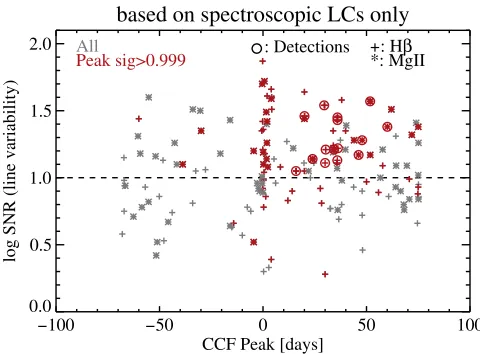
To demonstrate that we are mostly detecting real lags instead of false positives based on our spectroscopic-only data, we show in Figure 3 all of the 100 lowest-redshift SDSS-RM quasars in the CCF peak versus line variability S/N plane, again focusing on the Hβand MgIIlines only. The gray points
show all the CCF peaks regardless of their significance (searched over a symmetric range of lags centered on zero). The red points show those with a statistical peak significance
greater than 0.999, which immediately reveals a preference of positive CCF peaks(N=55)over negative(N=12)ones(i.e., lags of the lines relative to the continuum, and not vice versa). Objects with larger variability amplitudes in the lines allow more straightforward lag detection (i.e., comparing the gray and red points), as expected. This demonstrates that our spectroscopic-only LCs are able to detect true lags. There is clustering of significant peaks around zero lag, which suggests that there are correlated errors in the continuum and line LCs from spectroscopy alone, and/or it reflects the difficulty of detecting lags shorter than the spectroscopic cadence (a few days). Our 15 reported lag detections are shown as red circled points, and they are located in a“comfortable”region(i.e., with a large variability amplitude and inconsistent with zero lag) consistent with being genuine lags. There appears to be a deficit of significant peaks around∼+10 days in Figure3, albeit with small number statistics. We suspect that this is due to the small gaps between dark/gray time and bright time in our spectro-scopic monitoring(Shen et al.2015a). If this were the case, we expect that the addition of photometric data points in bright time would help recover the lags missed there. On the other hand, our reported lags are all longer than 10 daysand hence should not be significantly affected by these small gaps, as also supported by our tests with JAVELIN (where the LCs are interpolated within these gaps with physically motivated variability models).
To further use Figure 3 as guidance to estimate the bulk false-positive rate among the 15 reported lags, we perform the following tests.
Thefirst test is a shuffled-epoch test, where we shuffle the LC epochs for each objectand perform the same exercise as in Figure3with real data. By shuffling the LC epochs, we destroy any intrinsic correlation, and the frequency of significant CCF peaks from these mock LCs provides one measure of the false-positive rate. We typicallyfind∼4 cases with a positive peak, a peak significance>0.999, and S NLC>10, out of 155 LC pairs(Hβ+MgII)of the 100 objects. More importantly, we do
not observe a preference of positive peaks over negative peaks, as expected from random correlations from temporally uncorrelated data. Given the actual number of positive CCF peaks that pass the statistical significance andS N/ criteria in real data(N=40), this test suggests that the bulk false-positive rate is~10%. Note that among the 40 significant and high-S/N positive CCF peaks in the real data, we only selected 15 as our reported detections, and this selection should further reduce false positives based on visual inspection.
[image:7.612.47.287.50.227.2]One may be concerned that the shuffled-epoch test does not capture the intrinsic variability characteristics of quasarsand hence may underestimate the false-positive rate. An alternative test is the shuffled-LC-pair test, where we pair the continuum LC of one object to the line LC of another object in our sampleand perform CCF analysis to determine the rate of false positives. This test, however, assumes that individual quasar LCs are sufficiently different that there is no intrinsic correlation in the inter-object LC pairs. In practice, this may not be the case, as different objects may show a similar dominant feature in their LCs(such as a single broad bump/ dip)over the limited monitoring period, and thus these inter-object LC pairs will be correlated more often than assumed. Hence, the false-positive rate inferred from this test should be treated as an upper limit. Essentially, this test requires a large number of objects to sample the diversity in stochastic quasar Figure 3.Diagnosis of lag detections with spectroscopic-only LCs. Gray points
show the CCF peaks against the S/Nof the line variability for the 100 lowest-redshift quasars in SDSS-RM for which we have processed with PrepSpec, focusing only on the Hβand MgIIlines. Red points show only those peaks with a statistical significance greater than 0.999, thus removing spurious peaks from low-quality LC data. There is an obvious preference towardpositive peaks (i.e., lags) in the high-significance peaks, indicating that these spectroscopic LCs are meaningful in detecting lags. Objects with larger variability amplitudes in the lines allow more straightforward lag detection
(i.e., comparing the gray and red points). There is an excess of zero-lag peaks, which reflects correlated errors in the continuum and line LCs from spectroscopy alone, and/or the difficulty to detect lags shorter than the spectroscopic cadence(a few days). Finally, the red circled points show our reported detections, which have a CCF peak statistical significance greater than 0.999, an S/N in the line variability greater than 10, and a measured lag inconsistent with zero at>1s(see Section2.2for details).
29
We found that in a few cases, JAVELIN reports substantially smaller error bars on the lags compared with our CCF analysis, which may represent an underestimation by JAVELINand/or an overestimation by our FR/RSS approach.
7
variability, in order to justify the basic assumption that these inter-object LC pairs are intrinsically uncorrelated.
We performed the shuffled-LC-pair test for all 100 objects, focusing on Hβand MgIIonly (15,336 inter-object LC pairs).
We found roughly equal numbers of positive and negative peaks (581 versus 523), with a peak significance>0.999and
>
S NLC 10, confirming the results based on the shuffl ed-epoch test. We also found that3.8% of these inter-object LC pairs lead to a positive CCF peak with p>0.999 and
>
S NLC 10. Given the number of real LC pairs (155)in the parent sample, we therefore estimate that ∼6 cases will manifest from uncorrelated LCs as passing the S/N and the peak significance criteria as for the real data. This is about 15% of the 40 cases we observed with real data, which is an upper limit as explained above.
Therefore, based on the shuffled-epoch test and the shuffl ed-LC-pair test, we consistently estimate a false-positive rate of
∼10%–15% among our reported lags. This false-positive rate is also roughly consistent with the estimation from our simula-tions using mock quasar LC data and the SDSS-RM sampling/ spectral quality(Shen et al.2015a).
The basic properties of these lags are summarized in Table1, and the spectroscopic LCs are provided in Table 2. There are nine Hβlags and six MgIIlags. As mentioned in Section1, we
do not consider multiple line detections in the same object in the current work, but we simply note that there are cases where more than one line hasdetected(and consistent)lags, while in other cases there is only one line detected, and the other lines show signs of a lag but will require further data and in-depth analysis(see Section4). The important aspects of multiple line detections in the same object and their implications for BLR structure will be the focus of successive publications.
Epochs 3 and 7 have much lower S/N than the other epochs in our data (see Table 2 of Shen et al.2015a). For these two epochs, the narrow-line emission is often too noisy to use as a reliable internalflux calibrator, and as a result the data points at these two epochs sometimes appear as significant outliers (albeit with large error bars)from the adjacent LC data points. The standard interpolated CCF method does not treat the errors in the LCs rigorously and may be significantly affected by these discrepant or noisy measurements. Therefore, in such cases, we remove these problematic epochs(primarily epoch 7, sometimes both epochs 7 and 3)and rely on the rest of the epochs for the lag measurement. We only reject these epochs when necessary(i.e., if they significantly degrade the CCF), as rejecting data in general will reduce the correlation by reducing the sampling of the LCs. These rejected epochs are identified with a“1”in the last column of Table2.
3. RESULTS
3.1. Lags, BH Masses, and the R–L Relation
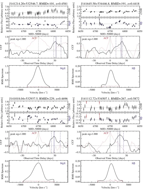
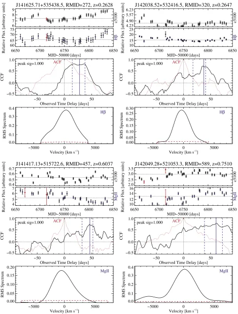
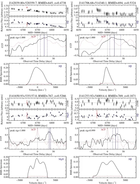
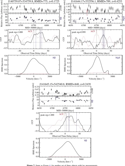
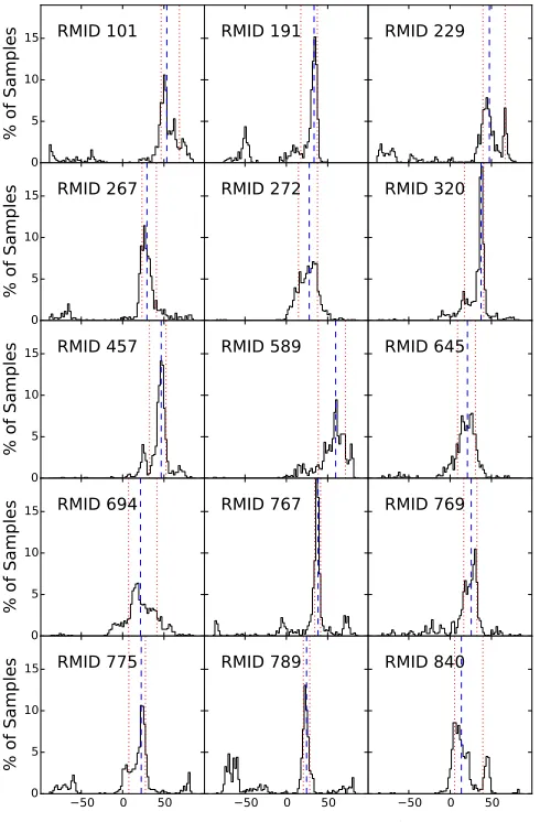
Figures4–7presentthe 15 lags in this work, where we show the LCs, the CCF, and the model rms broad-line profile for each detection. The autocorrelation function (ACF) of the continuum LCs is also shown for comparison with the CCF. We also show the CCCDs of these lag measurements in Figure 8. In all cases, there is a reasonably welldefined primary peak in the CCCD for us to determine the best lag and associated uncertainties. In a few cases there are substructures that are possible aliases owing to the sparse sampling of the
LCs. These substructures in the CCCD tend to increase the uncertainties in the lag measurements.
We consider these detections as preliminary, with the expectation that adding photometric LCs in our future work will significantly improve these detections(or falsify a small fraction of them, if any). We measure the broad-line dispersion srms (the second moment) and its uncertainty from the rms
spectra Bℓ( )l (continuum and narrow-line flux modeled and
subtracted in individual epochs) produced by PrepSpec. The mean continuum luminosity at restframe 5100 Å,
l
º l
L5100 L∣5100 Å, is measured from a multifunctional fit to
thefinal co-added spectra of all 32 epochs(Shen et al.2015a) that models the continuum, broad FeII emission and broad
+narrow-line emission (e.g., Shen et al. 2008). We have estimated the fraction of host starlight contributing to L5100
using a spectral decomposition approach described in Shen et al.(2015b)and derived the AGN-only continuum luminosity whenever the decomposition is physically meaningful(i.e., the host fraction is nonnegative at 5100 Å). This last step is important in deriving an unbiased BLR size–luminosity(R–L) relation for low-redshift AGNs with significant host contam-ination(e.g., Bentz et al.2013).
We compute a virial product(VP)using the measured time lag and rms line width:
t s
= c G
VP cent rms, 5
2
( )
wherecis the speed of light andGis the gravitational constant. The RM BH mass estimate is related to the VP asMRM=fVP, wherefis the average geometric factor(the virial coefficient)to account for the difference between line width and the virial velocity (e.g., Shen 2013; Peterson 2014). The value of f is usually determined empirically using the local BH mass–bulge stellar velocity dispersion(s*)relation and measurements ofs* in a subset of RM AGNs(e.g., Onken et al.2004; Graham et al. 2011; Park et al.2012a; Grier et al.2013b; Ho & Kim2014). We adopt a fiducial value of f=5.5 for this work (Onken et al. 2004), which is consistent with the latest work (Ho & Kim2014). We emphasize that this is the averageffactorand does not capture the diversity in the orientation and BLR structure in AGNs (e.g., Shen & Ho 2014; Pancoast et al.2014). The scatter in the actual virial factor for individual objects is currently a large contributor(a factor of 2–3)to the overall systematic uncertainty in RM BH masses (e.g., Peterson2014).
We can also compute a single-epoch(SE)BH mass estimate using the quasar continuum luminosity and the broad-line Hβ FWHM measured from the mean spectrum:
= + + b b - - ⎛ ⎝ ⎜ ⎞ ⎠ ⎟ ⎛ ⎝ ⎜ ⎞ ⎠ ⎟ ⎛⎝⎜ ⎞ ⎠ ⎟ M M
a b L
log
log
10 erg s 2 log
FWHM
km s , 6
SE,H
51000,tot 44 1
mean,H
1 ( )
Table 1
Basic Properties of the Lag Detections
RMID SDSS Designation Redshift Morphology Line srms,line tcent log VP f5100 logL5100 fhost FWHMmean,Hb logMSE,Hb smean,line FWHMrms,line hhmmss.
ss±ddmmss.s (km s-1) (days) (M) (10-17erg s-1cm-2Å-1) -erg s 1
( ) (km s-1) (M) (km s-1) (km s-1)
(1) (2) (3) (4) (5) (6) (7) (8) (9) (10) (11) (12) (13) (14) (15)
101 141214.20+532546.7 0.4581 point MgII 1167±9 36.7-+4.810.4 6.989-+0.0570.123 3.998±0.005 44.365±0.001 0.09 2443±12 7.889±0.004 1029±4 2391±46 191 141645.58+534446.8 0.4418 extended Hβ 990±19 23.3-+11.22.7 6.648-+0.2090.053 0.842±0.015 43.646±0.008 0.48 2173±34 7.550±0.014 838±12 1854±70 229 141018.04+532937.5 0.4696 extended MgII 1630±24 32.3-+5.312.9 7.225-+0.0720.174 0.575±0.004 43.551±0.003 0.49 3854±331 8.003±0.075 1582±20 3101±76 267 141112.72+534507.1 0.5872 point Hβ 1221±36 18.6-+3.87.1
-+
6.733 0.0920.169 1.078±0.004 44.092±0.002 0.39 2680±61 7.921±0.020 1403±6 2089±77 272 141625.71+535438.5 0.2628 point Hβ 1636±11 21.9-+10.47.9 7.059-+0.2050.157 6.190±0.254 43.929±0.018 0.00 2983±51 7.824±0.017 1515±2 3752±93 320 142038.52+532416.5 0.2647 extended Hβ 1362±33 29.6-+15.72.5
-+
7.030 0.2320.042 1.900±0.007 43.424±0.001 0.47 4462±114 8.057±0.022 1576±9 2975±64 457 141417.13+515722.6 0.6037 point MgII 1672±60 29.1-+8.83.6 7.201-+0.1350.063 0.188±0.005 43.366±0.012 0.60 4505±541 8.101±0.105 2574±39 3874±86 589 142049.28+521053.3 0.7510 point MgII 2824±33 34.0-+12.06.7 7.724-+0.1540.086 1.132±0.006 44.416±0.002 0.20 4750±117 8.521±0.021 3283±22 4108±39 645 142039.80+520359.7 0.4738 point Hβ 1360±20 14.2-+8.16.5 6.711-+0.2470.200 2.026±0.004 44.109±0.001 0.12 4122±58 8.222±0.012 1571±7 3696±55 694 141706.68+514340.1 0.5324 point Hβ 743±24 14.1-+9.512.9 6.183-+0.2920.398 1.635±0.004 44.155±0.001 0.23 1888±18 7.595±0.008 864±3 1661±104 767 141650.93+535157.0 0.5266 extended MgII 1394±10 25.1-+2.62.0 6.979-+0.0450.035 1.004±0.002 43.930±0.001 0.00 2088±94 7.514±0.039 1341±4 4066±202 769 141253.92+540014.4 0.1871 extended Hβ 1758±22 21.5-+7.75.8 7.114-+0.1550.117 1.563±0.010 42.972±0.003 0.72 4192±109 7.920±0.023 1769±13 5120±130 775 140759.07+534759.8 0.1725 extended Hβ 1790±10 19.2-+12.84.3 7.079-+0.2900.098 7.023±0.008 43.541±0.001 0.44 3661±33 7.933±0.008 1615±5 5115±59 789 141644.17+532556.1 0.4253 extended MgII 1371±27 17.2-+2.72.7 6.799-+0.0710.071 1.020±0.005 43.685±0.002 0.27 4128±138 8.052±0.029 1328±13 2681±96 840 141645.15+542540.8 0.2439 extended Hβ 1902±20 10.9-+6.620.9
-+
6.888 0.2610.832 1.321±0.007 43.178±0.002 0.67 5923±191 8.287±0.028 2492±29 4981±97
Note.Col.(1): object index in the full SDSS-RM sample described in Shen et al.(2015a). Col.(2): object designation in J2000 coordinates. Col.(3): redshift. Col.(4): object morphological classification based on SDSS imaging. Col.(5): the broadline used for the lag detection. Col(6): broad-line dispersion(second moment)for the line specified in col.(5)measured by PrepSpec using the rms spectrum. Col.(7): rest-frame time lag from the centroid of the CCF peak. Col.(8): virial product defined in Equation(5), which can be converted to the RM-based BH masslogMRM=log VP+logf withf=5.5 adopted in this work. Col.(9): observed
quasar continuumflux(host-corrected)at restframe 5100 Å, measured from spectralfits to the mean spectrum. Col.(10): quasar continuum luminosity(hostcorrected)at restframe 5100 Å. Col.(11): host-to-total fraction in 5100 Å continuum luminosity, estimated using a spectral decomposition approach(Shen et al.2015b). Col.(12): Hβbroad-line FWHM measured from the mean spectrum. Col.(13): single-epoch BH mass estimate based on the HβFWHM and continuum luminosity measured from the mean spectrum, using the formula from Vestergaard & Peterson(2006). Col.(14): broad-line dispersion for the line specified in col.(5) measured by PrepSpec using the mean spectrum. Col.(15): broad-line FWHM for the line specified in col.(5)measured by PrepSpec using the rms spectrum. All uncertainties presented here are 1σstatistical errors only. (This table is available in machine-readable form.)
9
The
Astrophysical
Journal,
818:30
(
17pp
)
,
2016
February
10
Shen
et
in our sample, we found that the SE masses based on Hβ are grossly correlated with RM masses with a scatter of∼0.28 dex, consistent with the results in Vestergaard & Peterson (2006) based on the local RM sample. However, there is a systematic offset of∼0.16 dex between the two sets of masses, indicating that there may be systematics when applying the Vestergaard & Peterson (2006) SE mass recipe to our objects at higher redshifts, or in the details of measuring the rms line widths. This minor discrepancy deserves further investigation with more RM results.
While not directly used for the calculations in this work, we also include in Table 1 measurements of the line dispersion measured from the mean spectrum and the FWHM measured from the rms spectrum for each line with a lag for completeness. These were measured from the PrepSpec models of the broad components of the Hβ and MgIIemission lines.
Two concerns with measuring the line dispersion are (1) the possibility of a bias introduced from blending in the wings with other emission components (see Denney et al. 2009)and (2) where to set the line boundaries. These are not a concern here because we are measuring the widths from the model profiles. This makes internally consistent measurements within our analysis, but they are model dependent and therefore may be difficult to reproduce if different assumptions are made for the spectral decomposition. BH mass estimates using alternative SE estimators can be obtained with the spectral measurements reported in Table 1.
Figure 9 shows the BLR size–luminosity relation (theR–L relation)based on the rest-frame 5100 Å quasar-only luminos-ity, where we compare our lag detections with the compilation of low-zRM results from Bentz et al. (2013). All low-z RM results are based on the Hβline. Our detections are atz0.3, but their locations on the R–L plot are consistent with those occupied by the low-z RM AGN sample within the uncertainties. The three most luminous objects with Hβ lags seem to fall below the localR–Lrelation(albeit with large error bars on the lags), which may be an indication that correlated errors in the continuum and line LCs from spectroscopy alone biased the lag measurements (see Section 2.2). Although the selection of the reported detections is not complete (see Section2.2), we did not intentionally choose detections that are consistent with the knownR–Lrelation, and hence there is no obvious bias from our selection of these detections. In addition, the several MgII lags seem to follow the same R–L relation
based on Hβ. The latter observation suggests that, at least in some quasars, there is overlap between the regions in which
broad MgIIand broad Hβoriginate(see also Sun et al.2015),
which is expected as both lines have similar ionization potentials. Of course, more data and analysis are needed to test this scenario.
The apparentflatness in theR–Lrelation for our detections in Figure9is mostly due to selection effectsand secondly due to the facts that the statistics and the dynamic range in luminosity for our sample are limited and that the lag measurement errors are substantial, rendering a potential correlation statistically insignificant. Given the sampling and duration of our spectro-scopic monitoring, we are most sensitive to lags on the order of tens of days (Shen et al.2015a). Shorter lags are difficult to detect given the sparse sampling of the spectroscopic LCs, while longer lags are difficult to detect given the limited temporal baseline. A more detailed analysis of theR–Lrelation based on SDSS-RM lag detections is beyond the scope of this work, which will require more lag detections and proper treatment of selection biases induced by our programand will be the focus of future SDSS-RM publications. For example, short lags may be recovered when incorporating more densely sampled photometric LCs, or at least upper limits can be placed and used in quantifying the R–L relation. On the other hand, simulations can be used to quantify the completeness in lag detections as a function of lag, given the parameters of the SDSS-RM program(Shen et al.2015a).
Finally, Figure 10 demonstrates the improvement of our results in the redshift–luminosity coverage of RM experiments. Our lag detections probe a new regime in this parameter space, providing RM measurements over approximately half of cosmic time. The median redshift is 0.03 for the local RM sample and 0.46 for our sample.
3.2. Additional Notes on Individual Objects
While our analysis demonstrates that the majority of these lag measurements are true detections, prior reverberation studies(e.g., Peterson et al.2004)indicate that when working with data that have low sampling rates, our lag detection methods can sometimes yield incorrect lag measurements despite reporting formally small uncertainties. The criteria for a robust measurement are difficult to quantify, and thus such classifications are somewhat subjective in nature, as they often rely on being able to “see” the reverberation signatures and having a narrow, well-defined peak in the CCF and/or CCCD. As such, our prior experience with RM leads us to identify a few of our lag measurements as lower-confidence measure-ments owing to various indicators, such as the lack of visible reverberation signatures in the LCs and/or a poorly defined or low peak correlation coefficient CCF. While our false-positive tests indicate that the detected time delays are likely real(and the lag measurements themselves are also supported using the JAVELIN method), we suspect that the accuracy of a few of the detections may be compromised for various reasons, despite the fact that they passed all of our statistical and quantitative tests for lag detections.
[image:10.612.43.294.74.107.2]The two targets where it is most difficult to evaluate the accuracy are RMID 229 and RMID 589. There are very few features visible in the continuum LC for RMID 229; the two most striking features are due to single epochs that are low S/N and were removed from several other targets owing to a suspect calibration, though they were not identified as outliers for this particular target. If the line LC is shifted by the best-determinedlag from our cross-correlation analysis to see Table 2
Continuum and Broad-line Light Curves
RMID MJD fcont econt fline eline Mask
101 56,660.209 5.959 0.008 33.151 0.511 0
Note.Continuum and broad-line light curves (time series of fluxes) are simultaneously derived from spectroscopy using PrepSpec(Section2.1), and the continuum is always estimated at restframe 5100 Å. Flux units are arbitrary. See Table 1 for the corresponding lines(Hβor MgII)and basic
properties of each object. The full content of the table is available in the online version. The errors on the LCs are the original PrepSpec output, while we have used inflated 3% fractional errors in the LCs in our CCF analysis (see Section2.2for details).
Figure 4.Light curves, CCF, and rms line profile for the 15 objects with lag detections. For each detection, the top panel shows the continuum(at restframe 5100 Å) and broad-line light curves, with the medianflux indicated by the dotted horizontal line. Bad epochs are marked in red and excluded from the CCF analysis(see text for details). The middle panel shows the CCF(solid black line), and theautocorrelation function(ACF)of the continuum LC is shown by the red dotted line. The lag
(i.e., the median of the CCF centroid distribution from FR/RSS; see Section2.2)is indicated by the solid vertical line, and the dashed vertical lines indicate the 1σ uncertainty in the lag. The statistical significance of the CCF peak is shown in the upperleft corner. The bottom panel shows the model rms broad-lineflux with the black line and the estimated errors with the red dashed line, both output by PrepSpec. We only show rmsflux errors within the adaptive broad-linefitting window, as errors outside thefitting window are not properly estimated in PrepSpec.
11
Figure 6.Same as Figure4, for another set of four objects with lag measurements.
13
whether the continuum and line LC features line up after this shift, the match is not extremely apparent, and the measured lag places many variability features observed in the line into gaps between observations of the continuum. In addition, the peak of the CCF is low (∼0.6). The CCF for RMID 589 is extremely broad and flat-topped; most of the correlation is driven by a long-term increase in flux over the entire set of observations rather than by shorter-term variability features that are more indicative of BLR reverberation. There is again a poor match with the continuum variability when the line LC is shifted by the measured lag.
For both RMID 191 and RMID 320, the correlation seems to be driven by either or both of the two possibly suspect epochs (epochs 3 and 7), and excluding those two epochs(at the cost of losing temporal sampling further) makes the correlation noticeably worse (albeit still formally consistent) in both of these targets. Again, when the line LCs are shifted by the measured time lag, the match is mediocre; the variability signal in the continuum of RMID 191 is rather low amplitude, and it is difficult to see similar features shared by both the line and
[image:15.612.47.292.51.424.2]continuum LCs. The peak of the RMID 191 CCF is also0.6, which is lower than that seen for our higher-confidence targets. RMID 694 and RMID 101 are cases that are somewhat marginalbut should be improved with the photometry and/or additional years of data. RMID 694 has inopportune gaps in the data; there is a gap in the spectroscopy in the middle of one of the major features of the LC that is potentially biasing the cross-correlation analysis—the incorporation of the photometry should resolve this issue. RMID 101 has a visible feature in the continuum that we only begin to see reverberated in the line when our campaign ended—thus, the lag measurement is likely more uncertain than it would be had we continued to observe for another month.
Figure 8.CCF centroid distributions(CCCDs)from FR/RSS for the 15 lags. The lags are in the observed frame to match Figures4–7. The vertical dashed and dotted lines indicate the reported lag and its uncertainties. In all cases there is a reasonably welldefined main peak in the CCCD to determine the best lag. In a few cases there are substructures (possible aliases due to the sparse sampling of the LCs)in the CCCD that will lead to elevated uncertainties in the lag.
[image:15.612.322.563.51.228.2]Figure 9.BLR size–luminosity relation. Our lag detections are shown as black circles(for Hβdetections)and red squares(for MgIIdetections). The data for previousz<0.3RM AGNs compiled in Bentz et al.(2013)are indicated with gray points. Our new lags are consistent with the locations of the previous RM AGNs used to calibrate the localR–Lrelation, but are not yet able to constrain theR–Lrelation independently given the limited numbers, precision, dynamic range, and possible selection biases inherent in our program(see discussion in the text).
Figure 10.Distribution of objects with detected lags in the redshift–luminosity plane. The red open circles are the 44 local RM AGNs compiled in Feng et al.
(2014), and the blue filled circles represent the 15 preliminary lag measurements in this work. Our lag detections probe a new regime in this parameter space, providing direct SMBH masses over approximately half of cosmic time.
15
[image:15.612.323.565.321.502.2]We anticipate that the ambiguities and concerns listed above will be resolved when the photometry and/or additional monitoring beyond the first six months is included in the analysis for these targets. Results for the remaining nine lag detections appear more robust; the LCs show a better match when the line LC is shifted by its measured time delay. In addition, they generally have higher peak correlation coeffi -cients in their CCFs(above 0.6), narrower and lessflat-topped CCFs, and, in most cases, the eye can pick out matching features in the continuum and line LCs that indicate a more robust, accurate lag measurement.
4. DISCUSSION AND CONCLUSIONS
From its theoretical definition by Blandford & McKee (1982), it took many years for RM to reach its current state, with some 60 local systems with well-measured lags, some-times for multiple emission lines (e.g., Peterson et al. 2004). RM studies of local AGNs are increasingly focused on detailed studies of individual objects to use the velocity dependence of the lags to study the structure of individual BLRs in detail(e.g., Bentz et al. 2010b; Grier et al. 2013a). It is not possible, however, to increase the overall size of the sample by an order of magnitude using the object-by-object approach that has been so successful to date.
The only way to increase greatly the sample size and to start to probe the UV emission lines of higher-redshift systems is to use the multiplex advantage of multi-object spectrographs. This has been explored theoretically in the contexts of both the SDSS using the SDSS BOSS spectrograph(Shen et al.2015a) and the Dark Energy Survey using the AAOmega spectro-graphs (King et al. 2015). These two studies emphasized slightly different goals but outlined the survey durations and cadences likely to yield transformative(100)numbers of new lag measurements across a broader range of luminosities, redshifts, and emission lines (e.g., Hβ, MgII, and CIV).
In both cases, these theoretical studies led to observational programs, and here we report initial results from the first year of spectroscopic observations in the SDSS-RM program. Compared to the predictions outlined in the theoretical studies, the allocated SDSS-RM spectroscopic observations alone for this first exploratory study appear subcritical, given the complexities in real LC data that were difficult to model in the simulations. On the other hand, the SDSS-RM program has obtained a large amount of supplementary photometric monitoring data from CFHT Megacam and the Steward Observatory Bok telescope that will be used to provide better sampled continuum LCs to compare with the line LCs from the spectroscopic data in our upcoming analyses. It is important, however, to show the results from simply analyzing the spectroscopic data alone for two reasons. First, even with this incomplete data set, we can measure a reasonable number of lags, thereby directly demonstrating the promise of the approach. Second, the yields based on spectroscopy alone are low and the uncertainties are great, as predicted by the theoretical studies for the as-obtained duration and cadence. It is desirable to increase the intensity of monitoring in order to have a significant yield of high-precision lag measurements in future multi-object RM programs.
In this study, we have presented preliminary lag measure-ments for 15 quasars at z<0.8 included in the SDSS-RM project, using the six months of 2014 spectroscopy alone. Our targets are fainter by 1–2 orders of magnitude than the local
AGNs that have been monitored for RM purposes, highlighting the difficulties of performing RM in this regime. Most of these lags are at z0.3 for intermediate-luminosity quasars, anL−z regime never explored in past work. These results demonstrate the general feasibility of our multi-object RM approachand provide some confidence for similar programs with multi-object spectroscopy (e.g., King et al. 2015). The lags are consistent with measurements used for local estimates of theR–Lrelations, but are not yet available in large enough numbers, precision, or dynamic range to improve on these local estimates. Several of them are, however, for the MgIIline, and
they demonstrate that MgIIdoes reverberate similar to Hβ. A
recent line variability study using SDSS-RM data also found that MgII does vary with similar (albeit slightly smaller)
amplitudes to Hβ(Sun et al.2015), as supported by the MgII
lag detections presented here. Moreover, we can see statisti-cally that we are close to measuring a much larger number of lags (see Figure 3). The problem is that with the present cadence and duration, there are many ambiguities in how to overlap the line and continuum LCs to produce an unambig-uous lag estimate unless the structure of the variations is optimal, and this occurs for only a small fraction of the targets withspectroscopic-onlyLCs.
For the present SDSS-RM program we will address this challenge in future papers by adding the better-sampled continuum LC data from our imaging programs (e.g., more than doubling the data points from spectroscopy). This should greatly increase the LC yield. Denser photometric LCs will enhance the cross-correlation signaland provide a remedy for correlated errors between the continuum and line flux measurements from spectroscopy.30Our preliminary investiga-tion on the photometric data showed great promises on this improvement.
It is also important to remind the reader that even for the small fraction of objects and the spectroscopic-only data we analyzed here, the reported lags are an initial demonstration rather than afinal conclusion on the yield of spectroscopic-only lags. There are many more formally detected lags based on the quantitative criteria in Section2.2that require refinements with photometric data. Moreover, we already see multiple-line lag detections in the same objects with this partial data set, as well as lags for other broad lines(such as Hα, HeII, etc.), but we
will defer such focused studies to upcoming SDSS-RM publications.
Extending the SDSS-RM program, particularly by adding more seasons of spectroscopic data, would also greatly improve the overall impact of the program. The SDSS-RM project continues to perform photometric and spectroscopic monitoring (albeit at reduced cadences) of the target field, which will strengthen the preliminary lag detections and reduce their uncertainties with more data. We have already observed another 12 spectroscopic epochs with the SDSS BOSS spectrograph in the 2015A semester(over six months)within the extended BOSS (Dawson et al. 2015), with twoepochs each month using a nominal exposure of 1 hr per epoch. Photometric monitoring in 2015 was carried out with a weekly cadence over the same period
30