A Random Forest Model for Predicting Allosteric and Functional Sites on
Proteins
Ava Sih-Yu Chen1, Nicholas J Westwood1, Paul Brear1, Graeme W Rogers 1, Lazaros Mavridis2 and
John B O Mitchell1*
1Biomedical Sciences Research Complex and EaStCHEM School of Chemistry, Purdie Building,
University of St Andrews, North Haugh, St Andrews, Scotland KY16 9ST, UK; and 2School of Biological
and Chemical Sciences, Queen Mary, University of London, London E1 4NS, UK
Email: Ava Sih-Yu Chen – [email protected] Nicholas J Westwood – [email protected] Paul Brear - [email protected]
Lazaros Mavridis - [email protected] John B. O. Mitchell - [email protected] * Corresponding author
Abstract
We created a computational method to identify allosteric sites using a machine learning method trained and tested on protein structures containing bound ligand molecules. The Random Forest machine learning approach was adopted to build our three-way predictive model. Based on descriptors collated for each ligand and binding site, the classification model allows us to assign protein cavities as allosteric, regular or orthosteric, and hence to identify allosteric sites. 43 structural descriptors per complex were derived and were used to characterize individual
protein-ligand binding sites belonging to the three classes, allosteric, regular and orthosteric. We carried out a separate validation on a further unseen set of protein structures containing the ligand
2-(N-cyclohexylamino) ethane sulfonic acid (CHES).
Keywords
1 Introduction
Allosteric regulation is the modulation of the activity of a protein, typically an enzyme, by the binding of a ligand molecule to a cleft other than the protein’s active site. A typical enzyme has one active site, but may have multiple allosteric sites.
The traditional understanding of allostery focuses on those binding events that induce a conformational change. The classical explanation of how allosteric regulation is achieved was proposed in the Monod-Wyman-Changeux (MWC) and the Koshland-Nemethy-Filmer (KNF) models,[1,2,3,4] where the cooperativity between subunits of an oligomeric protein is coupled with a
conformational change. According to the MWC model, cooperativity is achieved by a concerted transition between two alternative states, the protein being in either the T (tense) or R (relaxed) state. For the KNF model, a binding-induced conformational change in one subunit is propagated sequentially among other subunits. Both models imply that the conformational change at the substrate binding site results from the transmission of a signal initiated by allosteric effector binding.[1]
Conformational state redistribution is a concept that has been proposed to explain allosteric regulation. The native protein appears to exist as a conformational ensemble near the bottom of an energy landscape funnel.[5,6] In contrast to the oversimplified classical models, Weber proposed that
the binding results merely in a population shift of conformational states which were experimentally proved to have an effect on function.[7] Population redistribution enriches certain pre-existing
conformations which were previously hardly seen due to low population. It is through the interconversion of the functional conformations that allosteric regulation is achieved.[8,9]
Thus, Del Sol et al. think of allosteric regulation as redirecting the levels of traffic on dynamic
communication pathways that already existed prior to effector binding, rather than establishing new pathways.[3] They note that allosteric regulation can occur in the absence of significant
conformational change, though some kind of communication between sites must take place. Allosteric modulation can involve very fine levels of influence over the level of protein activity, whereas directly addressing the active site leads to a coarser granularity of control. They liken this to the contrast between allostery as a dimmer switch versus conventional orthostery as a simple on-off device.[3]
properties with the natural substrate, as a site distinct from the active site is targeted. This provides an alternative route for the discovery of promising new leads for regulation of the same target. Allosteric sites on proteins are also subject to lower evolutionary pressure compared to the active site, which is beneficial when designing target-specific inhibitors.
Despite the advantage of variation among homologs that an allosteric site has, this may cause difficulty in studying allosteric mechanisms, since the allosteric sites are hard to predict by traditional homology methods based on sequence similarity.[10] For protein families where a
reasonably large number of sequences are available, a more effective approach to sequence-based allosteric site prediction is to assume that allosteric sites are associated with networks of co-evolving residues.[11,12] In this way, Novinec et al. [13] identified a network of co-evolving residues putatively
responsible for communication between allosteric and functional sites from a multiple sequence alignment of papain-like cysteine peptidases. This prediction, along with associated experimental work, allowed them to identify a promising inhibitor candidate.
Other studies relevant to the prediction of allosteric interactions focus on simplified models of protein dynamics, using approaches like normal mode analysis (NMA),[10] energy exchange,[14] and
Monte Carlo path generation.[15] Panjkovich and Daura applied NMA to consider changes in the
flexibility of a protein upon ligand binding.[16] To achieve this, ligands were represented as dummy
atoms arranged in an octahedron. For each putative binding site, the NMA-derived B -factors of the apo and the bound states were compared in order to identify any large changes in the B-factors, these indicating potential allosteric sites.
A two-way classification model was proposed to differentiate allosteric from non-allosteric sites by Huang et al. [17] They developed a support vector machine (SVM) based machine learning model,
based on 90 allosteric sites selected from allosteric database (ASD) and1360 predicted non-allosteric sites from the same set of proteins using the Fpocket algorithm. This is distinct from our three-way predictive model containing two classes other than allosteric. For their SVM model, sets of site descriptors were derived to characterize the topological structure and physicochemical properties of both types of sites, obtaining a total of 41 site descriptors. A somewhat related method has been adopted by van Westen[18] et al. to select allosteric modulators based on the physicochemical and
structural descriptors calculated for those molecules from the ChEMBL database.[19] That approach
In this work, we focused on identifying potential allosteric sites, while making better use of available crystal data in the PDB. Almost all protein crystal structures contain non-cognate bound ligand molecules, such as stabilising agents and buffers used during crystallisation. We used the
co-crystallised ligands to calculate descriptors from the ligand and from the structures of the sites, thus building a machine learning model. Our aim is to identify binding sites which are purely crystal contacts from potential allosteric sites. These bound ligands could be a starting point to guide experiments aimed at probing the nature of the sites. To do this, we use a complementary approach, founded on a deeper analysis of the structures of potential binding sites. We assemble collections of three kinds of site based on its function: first, known orthosteric functional (active) sites of proteins in which the main cognate ligand binds; second, allosteric sites in which allosteric effectors can bind; third, a structurally representative set of other protein clefts, expected to be neither functional nor allosteric. For these three sets of sites, descriptors are proposed to identify and discriminate the binding state of individual ligands between the three different subsets. We use our existing protein-ligand scoring function RF-Score[22] and a new accessibility-like algorithm called CavSeek to
compute structurally-based binding descriptors and descriptors pertaining to the composition and flexibility of the clefts. We use these as features in a ternary predictive model, employing the Random Forest[23] machine learning algorithm. We take advantage of the out-of-bag data,[24] and
2. Methods
2.1 Random Forest
A Random Forest (RF)[23,24] is, as the name suggests, an ensemble of stochastically built decision trees
used for classification, or indeed for regression. Random Forest is widely considered relatively immune to overfitting. Each tree is grown by stochastic recursive partitioning, and the individual trees carry independent information because of the substantial random element in their
construction.
Every decision tree in the forest is firstly randomised using a bootstrap sample of Q instances from the training data, chosen by sampling with replacement from the Q objects in the training set. Thus, each object may be selected one or possibly more times for a given tree’s dataset, while about 37% of the instances remain unchosen in any particular bootstrap sample and constitute the so-called out-of-bag (OOB) data. The OOB data may serve as an internal validation set for the given tree. The combined performance on the separate OOB datasets of each tree can be aggregated, and
constitutes a fair test of the overall predictive performance of the Random Forest.
Secondly, each tree is randomised by permitting it to use, at each node, only a random subset of the features. At each node, a new subset of mtry features is chosen and the optimum split is created based on the best partitioning that is possible according to the Gini criterion,[25] using any single
valued attribute from a randomly chosen subset of mtry descriptors. As the training instances pass through the tree, they are therefore partitioned into similar sets, and each terminal leaf node becomes associated with a group of instances with homogeneous class labels.
Binary or multi-class classifications are determined by majority vote amongst the trees. For
classification, mtry is set by default to the square root of the number of descriptors, as it was in this work.[24] For the relatively small dataset and few descriptors used here, RF calculations are
inexpensive, and we chose to set the number of trees, ntree, to 10,000. Nonetheless, the improvement in prediction accuracy with additional trees above a typical ntree value of 500 is probably small.
Three further considerations apply to the use of Random Forest in this work. First, each tree is built by bootstrap sampling from the same balanced dataset, which we constructed by stratified sampling to include an equal number of objects (53) from each class, a total of 159 sites. Further, the
(balanced) dataset. Finally, Random Forest is designed to handle the inclusion of redundant and irrelevant descriptors through the process of selecting possible splits at each node from a substantial set of randomly chosen options.[24] This obviates any need for an explicit descriptor selection step,
and is particularly useful when a bespoke descriptor set is used, as in the present work.
2.2 CavSeek
In order to measure the burial of a ligand within the cavity of the protein binding site, we developed an accessibility-like program called CavSeek using a script written in Java. For a given protein and ligand, we calculate the percentage of possible point-to-atom contacts which are shorter than a given threshold value and hence are said to be “in contact”. A number of thresholds from 0.5 to 2Å have been selected to profile optimally and identify a ligand’s binding site. The aim of this program is to make it possible to discriminate computationally between surface-binding molecules and
pocket-binding molecules. Ligands that are found within a protein cleft in a small binding pocket will have a higher percentage of sub-threshold contact distances. The percentage burial increases with the size of the thresholds as more points are counted. To generate descriptors from CavSeek, one can either include the result at each different threshold as a separate descriptor, or calculate an average burial as a single descriptor. For this study, we have included the burial at nine individual thresholds and also the average burial.
In detail, CavSeek first centres the protein-ligand complex at the geometric centre of the ligand. We remove all protein atoms which are more than 20Å away from this origin, since there is a very little prospect of those atoms having a significant interaction with the modestly sized ligands that we study. We then represent each ligand atom as a sphere using the following van der Waals radii (r) in Å: Br (1.85), C (1.7), Cl (1.75), F (1.47), Fe (2.0), I (1.98), N (1.55), O (1.52), P (1.8) and S (1.8).[26] For
2.3 RF-Score
RF-Score[22] is our group's machine learning approach to predicting protein-ligand binding affinity,
especially for docked structures. Previous knowledge-based approaches used ensembles of observed protein-ligand crystal structures to infer binding energies from atom-atom distance distributions. That approach makes the dubious assertion that Boltzmann energetics apply, assuming a particular exponential functional form to transform distance distributions into binding energies.[27] RF-Score
uses Random Forest to predict binding affinities from both structural data and the affinity data that are left unused in most knowledge-based approaches, yielding a much more accurate and flexible scoring function.
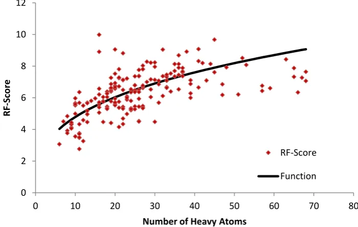
In order to make the scores of differently sized ligands comparable, and to compensate for the intrinsic size-dependency of scoring functions, we calibrate RF-Score according to the number of heavy atoms (N) of its ligand.[28,29] Figure 1 illustrates the variation of the unadjusted scores, which
we empirically fitted to a small number of physically justifiable functional forms. We empirically found that the best fitting function defining the expected score (E) for a ligand of given size was
E = 2.222 N1/3
[image:8.595.87.438.477.699.2]For each ligand, we calculate the unadjusted RF-Score (R), the expected score (E), and the normalised score (R/E).
Figure 1 – Normalisation of RF-Score
0 2 4 6 8 10 12
0 10 20 30 40 50 60 70 80
RF
-S
co
re
Number of Heavy Atoms
Each point represents an individual RF-Score of a different protein-ligand complexselected from the PDBbind database[28] used in this study as part of the subset of orthosteric sites within the training
set. The fitted curve illustrates the function used to calibrate the scores with the ligand size.
2.4 Temperature Factor
To include features that describe flexibility, we have used the temperature factor (or B-factor). The B-factor, which reflects the degree of atomic displacement from their equilibrium positions in the crystals due to thermal motion, was extracted from the X-ray crystallographic structures of the protein-ligand complexes in the PDB. A higher B-factor implies that the atom has greater mobility. The average B-factor of the contact residues is divided by that of the protein to obtain values that reveal the differences in flexibility of the ligand binding region with respect to the entire protein. Firstly, to consider the bias arising from chain termini; the average B-factor of the protein with gradual omission of up to 10 residues at both ends was calculated. The results showed no significant change in the average B-factor between each omission; accordingly proteins have been kept without terminal elimination. Secondly, the solvent and other ligands or cofactors were removed to obtain a B-factor resulting solely from the protein residues. The contact residues herein were defined as residues having at least one atom within 4Å of the centre of any atom of the ligand. B-factors of all the atoms of the contact residues and the protein are averaged and were included both as ratios and as separate descriptors in this study.
2.5 Contact Residues
2.6 Small Molecule Descriptors
We used the Chemistry Development Kit (CDK)[30] to compute descriptors for small molecules. CDK is
an open source library written in Java for structural informatics calculations. First, the chemical structures of the ligand were inputted as SMILES extracted from each ligand structure file (in SDF format). Second, we calculated 277 CDK descriptors for each compound, and removed features without discriminant power, those having either the same or an undefined value for all compounds in any of the training subsets. As a result, only the remaining 141 CDK descriptors were kept for further analysis.
Table 1 - List of descriptors and their abbreviations
RFSCxCSK The RF-Score (R) times average burial over nine thresholds estimated by CavSeek
Binding Site
RF.score The unadjusted RF-Score (R) Binding Site
NormRFScore The normalised RF-score (R/E) Binding Site
Function_F195 The expected RF-score (E), calculated by a fitting function E=2.222 N⅓
Binding Site
B_protein Average B-factor of the protein Binding Site
B_pocket Average B-factor of the contact residues defined as protein residues <4Å to the ligand
Binding Site
noContact_resi Number of contact residues Binding Site
2.7 Dataset
2.7.1 Allosteric Sites
A total of 91 proteins adopted from Panjkovich and Daura’s work were initially used to represent the subset of allosteric sites in the training set.[10] The data were primarily collected from the online
AlloSteric Database (ASD) and from the literature, and were further filtered to be structurally non-redundant by the sequence clustering program BLASTClust. The protein with the highest resolution structure of each of the resulting 91 groups was selected to represent that group. ASD[31]
provides a list of the allosteric residues in the given protein. We compared those residues, thus annotated as comprising an allosteric site, to the list of residues involved in ligand binding extracted from PDBsum.[32] From this, we can identify any ligand that is bound in the allosteric site in order to
obtain descriptors which capture the binding profile of the ligand in the allosteric pocket. If there are many instances in which the same ligand adopts an equivalent binding mode, the one with the highest RF-score value is kept in the subset to represent the particular binding pattern. Thus, the list has been whittled down to 59 representative allosteric (A) protein pockets.
2.7.2 Regular Sites
The regular site subset was derived from a representative set of protein domain structures, each of which is given by CATH[33] as an example representing the homologous superfamily to which it
belongs. From each such structure, one ligand binding site is selected according to PDBsum.[32] For
enzymes, we choose sites having a ligand which is neither a cofactor nor similar to the enzyme’s product or substrate. Ligands were selected to have no contact with any residues of any allosteric site given in ASD. Therefore, the sites occupied by the selected ligands are unlikely to be active sites or allosteric pockets. The regular subset is expected to have the weakest binding affinity and the lowest burial value of the three subsets. These weak interactions correspond to the regular binding events by which non-cognate ligands bind, possibly as accidents of crystallisation.
A total of 99 instances were selected for the subset of regular (R) sites. The number representing each class was designed to be proportional to the prevalence of that structural class amongst all CATH[33] superfamilies (2620 superfamilies in total). There are four top C-level classes defined in the
Table 2 - Distribution of regular sites amongst CATH C-level classes
Class No.
Mainly alpha 32
Mainly beta 20
Alpha beta 42
Few Secondary Structures 5
2.7.3 Orthosteric Sites
A total of 195 protein-ligand complexes representing the subset of orthosteric (T) sites were retrieved from the PDBbind database (version 2007).[34] These data were originally used for the
purpose of validating scoring functions in Cheng et al.'s study.[28] The data contain experimentally
determined binding affinity values obtained from the literature. Cheng et al. further filtered their initial collection of data to account for the quality of structures, the quality of binding data, the components of complexes and redundancy of protein sequences, to avoid over-representing certain families. They clustered the remaining complexes according to sequence similarity and selected the complexes with the highest, the median and the lowest binding affinity to represent each of the 65 clusters, giving 195 complexes in total. In this study, we have further whittled down the number to 159 complexes which have only small molecules in the pocket.
2.7.4 Datasets for Tree Building and Validation
The Random Forest class predictions are probabilistic and subject to potential sources of error. The Gini splitting rule, based on reduction of node impurity, tends to isolate the largest class to produce a pure node. Accordingly, there will be a bias produced due to unbalanced class sizes. A class with fewer data is less likely to be correctly assigned. One way to reduce this size-related effect is to weight the training set inversely proportionally to the size of the class, however, this in turn causes a higher rate of misclassification. The other way is to even up the number of samples in each class.[35,36]
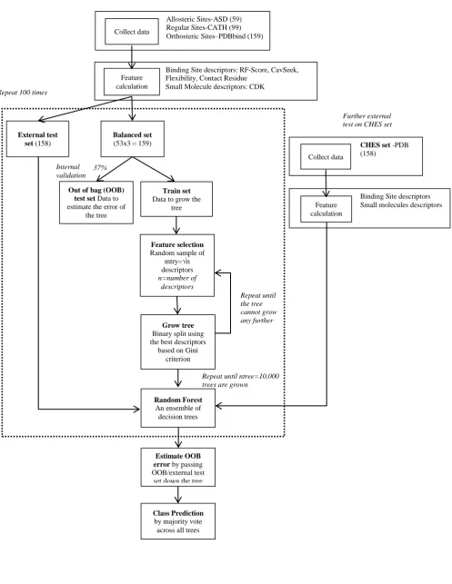
constructed tree, and the remaining 37% ( 1/e) or so are reserved for OOB validation of that tree. The bootstrap sampling from the balanced set is repeated afresh for each of the 10,000 trees. In this work, those data excluded from the stratified balanced set in advance of the bootstrap sampling form an external test set which was separately used for further validation. This entire process of generating 10,000 trees was itself repeated a hundred times with different random seeds to avoid losing information from the majority class in training the models, see Figure 2.
2.8 CHES as a Ligand
The PDB crystal structures containing the buffer molecule CHES (2-(N-cyclohexylamino) ethane sulfonic acid) were investigated. CHES is one of the many buffer molecules that commonly complex with proteins during the crystallization process, despite their role in maintaining protein solubility and stability for NMR experiments.[37] Yet growing evidence of its effect on protein dynamics implies
that protein function will be affected by ligand binding.[38] These molecules can be used as a starting
point for designing novel probes for new allosteric sites and as a tool to study changes in protein dynamics induced upon the binding of a buffer molecule.[39] In this study, buffer molecules are
introduced as potential binders to identify locations of possible allosteric sites.
In total, 82 CHES containing entries had been released in the PDB up to Dec 2013. From these, our external validation CHES set of 158 CHES-protein binding sites (some proteins have multiple CHES ligands) has been identified and each site is characterized by a set of descriptors individually
calculated for it. We noted 14 cases in which CHES was bound in a protein's defined pockets,[39] from
which only one of these 14 CHES molecules was found in an allosteric site, that of a bacterial sialidase (NanB).[40] There results were manually identified by Brear and Westwood,[39] who were
Figure 2 – Flowchart of the model development scheme
Allosteric Sites-ASD (59) Regular Sites-CATH (99) Orthosteric Sites–PDBbind (159)
Binding Site descriptors: RF-Score, CavSeek, Flexibility, Contact Residue
Small Molecule descriptors: CDK
Balanced set
(53x3 = 159) Feature calculation
Train set
Data to grow the tree
Out of bag (OOB)
test set Data to
estimate the error of the tree
Random Forest
An ensemble of decision trees 37%
Collect data
Feature selection
Random sample of mtry=√n descriptors n=number of
descriptors
Grow tree
Binary split using the best descriptors
based on Gini criterion
Estimate OOB
error by passing
OOB/external test set down the tree
Repeat until ntree=10,000 trees are grown
Repeat until the tree cannot grow any further
CHES set -PDB
(158) Collect data
Further external test on CHES set
Binding Site descriptors Small molecules descriptors Feature
calculation Internal
validation
Class Prediction
by majority vote across all trees
3. Results and Discussion
3.1 Predictive performance
Prediction is based on a majority vote over the set of 10,000 trees. One vote is made by each tree for each instance that is OOB (not used in building the tree, because it was not chosen during the bootstrap sampling) by passing the OOB data down each tree to obtain a class prediction. From the aggregated OOB predictions, classes are assigned to each OOB instance by a majority vote of the trees. The OOB error, which shows the percentage of misclassification in the dataset, was calculated based on the known and predicted class labels. Separately, we also test the Random Forest’s
predictivity by passing down each tree the external test set comprising those data that were omitted from the balanced set (46 R, 106 T and 6 A sites).
Random forest is insensitive to values of mtry except close to its high and low extreme values.[41] For
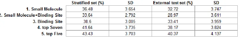
all 100 repeats (each of 10,000 trees per model), the default mtry was used. Five models were built using various sets of descriptors, which are classified as either small molecule or binding site descriptors according to the physicochemical features captured. Some of the most significant descriptors are listed in Table 1. For each model, we computed the average OOB error to estimate the prediction error; see Table 3.
The OOB error is sensitive to the random determination of which protein-ligand complexes are kept in the training set, in general, with 3-4% deviation from the average. The first Random Forest model was trained using a total of 151 small molecule descriptors including 141 CDK descriptors and the heavy atom counts of each ligand. The average OOB error of the Random Forest models obtained is 36.48% on the stratified balanced set, in which the pocket has been assigned a class label solely based on the small molecule descriptors of the ligand that binds to it. By the addition of 43 binding site descriptors, the second Random Forest model which includes properties of all calculated descriptors of both the bound ligand and the site has a slightly improved error of 33.64%. Both models contained descriptors based on the structures of the small ligand molecules. These are invariant within the CHES set as the same compound CHES was used to characterise the pocket in each case. Thus, those models are not used in predicting our CHES set since these are descriptors without discriminating power for that set.
Subsequently, it was used on the CHES set to generate predictions for the CHES-protein binding pockets.
Table 3 - Average OOB error rates for the different models.
The OOB errors are presented as the percentage of misclassified data points in the stratified balanced set and separately in the external test set (comprising data excluded from the stratified set). Standard deviations are calculated over a hundred runs using different random seeds (10,000 trees per run), using N-1 = 99 in the denominator.
3.2 Descriptor Importance
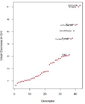
The importance of the individual descriptors can be evaluated either with the permutation method by observing the effect on the predictivity of Random Forest models of ‘noising up’ each descriptor in OOB data, or alternatively with the Gini index, an impurity measure. The mean decrease Gini (MDG) (calculated over all trees) is a measure of improvement to the purity when that descriptor is made available to split the trees, thus producing greater purity in the resulting nodes. The decreases in Gini impurity for each descriptor used to form splits are summed over all trees and then
normalised. A higher value implies greater importance of the variable concerned. Here, we report the results of variable importance as measured by impurity reduction, see Figure 3.
The top ranked binding site descriptors obtained by averaging the Gini importance values from 100 repeats are obtained. The leading descriptors are: first the product of the RF-Score and the average score of CavSeek (RFSCCSK), second the RF-Score values (RF.score), followed in third place (but with a significant decrease in importance) by protein flexibility (abbreviated to B_protein), fourth the residue count of the ligand binding site (noContact_resi), and fifth the normalised RF-Score
(NormRFScore).
the number of heavy atoms N to the original score as 2.222N⅓). Those two have very similar Gini
importance values.
Similar importance rankings were found in all hundred repeats, but they sometimes slightly differed in order. The calculation of relative importance allows a further assessment firstly of the classifiers based on the full set and secondly on classifiers based only on a few of the most important
descriptors as a potential way to improve the performance. To achieve this, we select the top 7 descriptors (from which to build the fourth model) and top 5 descriptors (for the fifth model) due to the breaks in the curve of the Gini importance plot, Figure 3, indicating a considerable drop of importance from the fifth to the sixth variables and similarly from the seventh to the eighth. The predictive ability of the models with reduced numbers of descriptors, as measured by the OOB error, is shown in Table 3. An increased overall OOB error is observed as the number of variables is
decreased by 3.04% and 4.83% for the stratified set, relative to the model based on all binding site descriptors. Apart from the OOB error calculated, we also look for consensus of the results of computational predictions and literature findings, as discussed below.
Figure 3 - The mean Gini importance values of each descriptor from the third model, averaged over a hundred repeats.
The plot shows variable importance on the y-axis ordered from the most to the least important. The descriptors with the highest decrease in Gini impurity make the major contributions to partitioning the data into homogeneous classes.
3.3 Predictions for the CHES set
The model trained using all binding site descriptors returns six orthosteric (T) sites, of which four (pdb codes: 2VW2, two sites in 3OQI, and 3NOQ) showed matches with the manual annotation. The remaining two were known bind to the domain interface (both in 2ICH) interacting with conserved residues which were inferred to have functional role among homologs.[42]
Among 15 CHES binding instance predict as allosteric (A), there is lack of literature for 4DQ0 and 3G8W. Both contain multiple CHES binding instances. Our results uncover three potential allosteric sites, which are not known orthosteric sites, supported by the literature. Four were found
experimentally in sites considered[39] likely to be orthosteric (two in 3RIG, 1Q1Q and 1V30), see Table
S1 (Supporting Information).
Since CHES is not a natural cognate ligand for any protein it binds to, it is perhaps not surprising that orthosteric sites where the CHES binds (active sites evolved to bind other ligands) have been
predicted as allosteric. The ligands in the orthosteric (T) subset of the training set from which the model was built were chosen to be more specific to the corresponding protein; thus, the more buried and stronger binding ligands were expected to be the cognate ones. In the potential future use of this methodology to predict allosteric sites using serendipitous binders, the workflow would therefore be designed to filter out known orthosteric sites from the set of allosteric predictions.
In contrast, our fifth model using the top 5 descriptors resulted in more promising results. Five orthosteric sites have been predicted of which four are consistent with the previously discussed full binding site descriptor model (2VW2, two sites in 2ICH, and 3OQI). An equal number of predictions amongst the 100 repeats assigned 3OQI to the orthosteric and allosteric classes. Three out of five orthosteric predictions were indeed experimentally determined to be orthosteric (2VW2, 3OQI and 1V30), while the remaining two are found at the domain interface (2ICH).
The top 5 descriptor model identified 30 allosteric sites, of which 15 lack definitive description in the literature, six pockets correspond to manually annotated orthosteric sites (two in 3RIG, and one in each of 1Q1Q, 3OB9, 3NIB, and 4H75), and nine pockets were potential allosteric sites. The allosteric sites we have referred to are non-orthosteric clefts, based on the literature. Yet, it is not known whether those pockets are functional allosteric sites, see Table S2 (Supporting Information).
Unfortunately, the allosteric site obtained manually (2VW2, A1001) by Brear and Westwood[39] was
We notice that three interface cavities were assigned to classes A or T (two in 2ICH, and 4ATG), implying that there may be shared features of interface interaction common to the allosteric and orthosteric subsets. Indeed, the interface can potentially act as a binding site for an allosteric modulator. Binding of allosteric modulators at the interface between subunits of GABA receptor has been shown to have varying effects on the receptor's function.[43] Stanget et al.[44] revealed an
allosteric binding site at the homodimeric interface of caspase-6 zymogen that impairs function. Descriptors to identify specifically the interaction interface can be exploited; perhaps interface cavities might be included in future work as an independent subset.
One positive note is that, in spite of high error rates (38.6% for the full binding site descriptor model and 43.43% for the top 5 descriptor model) estimated using OOB data, both models have given promising results for potential allosteric sites. Nearly half of our prediction instances are not
confirmed by the literature, yet instances that can be found in the literature are annotated as either orthosteric or in a binding cavity different from the orthosteric site. In fact, our top 5 descriptor model predicts most of the defined pockets (10 out of 14) that have been identified by Brear and Westwood to be either allosteric or orthosteric.
Our method provides a fast and low computational cost way to identify potential allosteric sites on large number of crystal structures. The co-crystallised non-cognate ligands and buffers that are commonly seen on most crystal structures are used, from which we extract binding site features. The predictions were made based only on structures with no cognate ligand bound. Thus, an adequate description of a binding cleft might not be possible. Also, potential allosteric sites
containing no co-crystallised compound are invisible to our trained algorithm. The models were not trained to predict based on specific families. Thus, the number of regular sites included for each of the four structural classes at the C-level of the CATH classification[26] is roughly proportional to its
prevalence in the CATH database. However, we noted that a known allosteric site is dominant in some families[18] or perhaps may only exist in particular families, thus introducing a systematic bias.
4. Conclusions
Allostery is a regulatory mechanism that affects protein function by the binding of small molecules to a site distinct from the active site. In contrast to traditional drug design by mimicking natural substrates, allosteric effectors offer therapeutic benefit for target-specific drug design. The discovery of new allosteric sites in protein cavities has emerged as a new drug design approach to identify novel pharmaceutical agents.
In this study, we have used Random Forest to build a three-way classification model for predicting allosteric pockets. We then report the results for a test set in which we consider instances of a buffer molecule, CHES, as a potential binder to allosteric sites; Brear and Westwood[39] observe 14 matches
supported by the literature and structural analysis, wherein 10 of these 14 pockets were identified as either the allosteric or orthosteric sites of the protein by our top 5 descriptor model. Although it is questionable whether other predicted pockets are truly functional, the implementation of a machine learning scheme allows discrimination between binding sites according to features that are captured from the protein-bound ligand conformations. This can help reduce the number of PDB files needing to be looked at when hunting for potential novel allosteric sites, prioritising those which are
predicted to belong to the allosteric category. Thus, this study shows promising results from using adventitiously binding buffer molecules as agents for allosteric site discovery. However, we also note that predictions of orthosteric pockets were hardly ever made for binding sites of CHES, a
non-natural ligand for any protein. CHES appeared to be associated with lower binding affinity and lower burial in protein cavities compared to the ligands of the orthosteric subset used in the model’s training. However, mispredictions of orthosteric sites as allosteric will be easy to remove from a set of allosteric predictions, since the orthosteric sites are generally known for the PDB structures we are using. We found several CHES molecules that were predicted to be either allosteric or
orthosteric sites are bound at an interface, which can potentially be allosteric modulator binding sites.
Supporting Information
Tables S1 and S2 compare the predicted based on the binding site and the top five descriptor model versus literature for each CHES binding instance. Only instances assigned to the allosteric (A) or orthosteric (T) classes are shown. The assigned pockets that were identified by Brear[39] have been
highlighted in italics. The results were ordered based on the number of predictions obtained for the assigned class from a hundred runs.
Competing interests
The authors declare that they have no competing interests.
Authors' contributions
SYC – Building the datasets, calculating the descriptors, writing the R scripts and running the models, SYC and JBOM – writing manuscript. NJW, PB and GWR - Generation of the original project concept and manual inspection of PDB files for comparison with computational results. LM – Writing the CavSeek software. JBOM and NJW – conceiving and supervising project.
Acknowledgements
References
[1] Tsai CJ, Del Sol A, Nussinov R, Mol. Biosyst.2009, 5, 207-216. [2] Gunasekaran K, Ma B, Nussinov R, Proteins2004, 57, 433-443. [3] Del Sol A, Tsai CJ, Ma B, Nussinov R, Structure2009, 17, 1042-1050. [4] Laskowski RA, Gerick F, Thornton JM, FEBS Lett.2009, 583, 1692-1698. [5] Boehr DD, McElheny D, Dyson HJ, Wright PE, Science2006, 313, 1638-1642. [6] Malmendal A, Evenäs J, Forsén S, Akke M, J. Mol. Biol.1999, 293, 883-899. [7] Volkman BF, Lipson D, Wemmer DE, Kern D, Science2001, 291, 2429-2433. [8] Kumar S, Ma B, Tsai CJ, Sinha N, Nussinov R, Protein Sci.2000, 9,10-19. [9] Tsai CJ, Ma B, Nussinov R, Proc. Natl. Acad. Sci. USA1999, 96, 9970-9972. [10] Panjkovich A, Daura X,BMC Bioinformatics2012, 13: 273.
[11] Lockless SW, Ranganathan R,. Science1999, 286, 295-299.
[12] Lu S, Huang W, Zhang J, Drug Discovery Today,2014, 19:1595-1600.
[13] Novinec M, Korenč M, Caflisch A, Ranganathan R, Lenarčič B, Baici A, Nat. Commun. 2014, 5:3287.
[14] Erman B, Physical Biology2011, 8: 056003.
[15] Kaya C, Armutlulu A, Ekesan S, Haliloglu T, Nucleic Acids Research2013, 41: W249-W255. [16] Panjkovich A, Daura X, Bioinformatics2014, 30:1314-1315
[17] Huang W, Lu S, Huang Z, Liu X, Mou L, Luo Y, Zhao Y, Liu Y, Chen Z, Hou T, Zhang J,
Bioinformatics2013, 29:2357–2359.
[18] van Westen GJ, Gaulton A, Overington JP, PLoS Comput Biol.2014, 10: e1003559. [19] Bento AP, Gaulton A, Hersey A, Bellis LJ, Chambers J, Davies M, Kruger FA, Light Y,
Mak L, McGlinchey S, Nowotka M, Papadatos G, Santos R, Overington JP, Nucleic Acids Res.2014, 42, 1083-1090.
[20] Greener JG, Sternberg MJE, BMC Bioinformatics 2015, 16:335
[21] Demerdash ONA, Daily MD, Mitchell JC, PLoS Comput Biol. 2009, 5: e1000531. [22] Ballester PJ, Mitchell JBO, Bioinformatics2010, 26, 1169-1175.
[23] Breiman L, Mach. Learn.2001, 45, 5-32.
[24] Svetnik V, Liaw A, Tong C, Culberson JC, Sheridan RP, Feuston BP, Journal of Chemical Information and Computer Sciences2003, 43, 1947-1958.
[25] Raileanu LE, Stoffel K, Annals of Mathematics and Artificial Intelligence2004, 41, 77-93. [26] Bondi A, J. Phys. Chem.1964, 68, 441-451.
[29] Kuntz ID, Chen K, Sharp KA, Kollman PA, Proceedings of the National Academy of Sciences USA,
1999, 96, 9997-10002.
[30] Steinbeck C, Han Y, Kuhn S, Horlacher O, Luttmann E, Willighagen E, J. Chem. Inf. Comput. Sci.
2003, 43, 493−500.
[31] Huang Z, Zhu L, Cao Y, Wu G, Liu X, Chen Y, Wang Q, Shi T, Zhao Y, Wang Y, Li W, Li Y, Chen H, Chen G, Zhang J, Nucleic Acids Res.2011, 39, D663–D669.
[32] Laskowski RA, Nucleic Acids Res.2001, 29,221-222.
[33] Cuff AL, Sillitoe I, Lewis T, Redfern OC, Garratt R, Thornton J, Orengo CA, Nucleic Acids Research
2009, 37, D310–314.
[34] Wang R, Fang X, Lu Y, Yang CY, Wang S, J. Med. Chem.2005, 48, 4111-4119. [35] Breiman L, Machine Learning1996, 24, 41–47
[36] Richards JW, Starr DL, Butler NR, Bloom JS, Brewer JM, Crellin-Quick A, Higgins J, Kennedy R, Rischard M, Astrophys. J. 2011, 733, 12-15
[37] Hardy JA, Wells JA,Curr. Opin. Struct. Biol. 2004, 14, 706-715 [38] Long D, Yang D,Biophys. J.2009, 96, 1482-1488
[39] Brear P, PhD Thesis, University of St Andrews 2012
[40] Xu G, Potter JA, Russell RJ, Oggioni MR, Andrew PW, Taylor GL, J. Mol. Biol. 2008, 384, 436-449 [41] Svetnik V, Liaw A, Tong C, Wang T, Lecture Notes in Computer Science2004, 3077, 334-343 [42] Chiu HJ, Bakolitsa C, Skerra A, Lomize A, Carlton D, Miller MD, Krishna SS, Abdubek P, Astakhova T, Axelrod HL, Clayton T, Deller MC, Duan L, Feuerhelm J, Grant JC, Grzechnik SK, Han
GW, Jaroszewski L, Jin KK, Klock HE, Knuth MW, Kozbial P, Kumar A, Marciano D, McMullan D, Morse AT, Nigoghossian E, Okach L, Paulsen J,Reyes R, Rife CL, van den Bedem H, Weekes D, Xu Q, Hodgson KO, Wooley J, Elsliger MA, Deacon AM, Godzik A, Lesley SA, Wilson IA, Acta Crystallogr. Sect. F Struct. Biol. Cryst. Commun. 2010, 66, 1153-1159.
[43] Sancar F, Czajkowski C, Neuropharmacology 2011, 60, 520-528