Abstract— Automobile companies have increased the use of high strength dual phase steels as an alternative to aluminium and magnesium alloys due to their light weight, low cost and durability. Due to their high tensile strength, however, dual phase steels have a tendency to springback more than other structural steels in a forming operation. In addition, variations in material properties and manufacturing process parameters cause springback variation over different manufactured parts. Therefore, it is an important task to reduce the magnitude of springback as well as its variation within to produce robust and cost-effective parts. This paper investigates minimization of the magnitude and variation of springback of DP600 steels in U-channel forming within a robust optimisation framework. The computational cost is reduced by utilizing metamodels for prediction of the springback and its variation during optimisation. Three different allowable sheet thinning levels are considered in solving robust optimisation problem and it is found that as the allowable thinning increases the die radius reduces thereby the magnitude and variation of springback reduces. Finally, a sensitivity analysis is performed and the yield stress is found to be the most important random variable.
Index Terms—Dual phase steels, metamodels, Monte Carlo simulations, robust optimisation, springback.
I. INTRODUCTION
pringback is one of the most important problems observed during sheet metal forming process. The deviation of the manufactured geometry from the designed geometry is called as springback. The high strength of dual phase steels leads to more springback than traditional steels. Moreover, variation of springback is another challenging problem to overcome. Variations in material properties and manufacturing process parameters are the main effects that cause springback variation. Large variation in springback limits the application of springback prediction and compensation techniques. Therefore, problems increase in the assembly of manufactured parts.
Manuscript received Jan 17, 2011; revised Mar 24, 2011. This work was supported by The Scientific and Technological Research Council of Turkey, under award MAG 109M078.
D. Bekar is with the Department of Mechanical Engineering, TOBB Economics and Technology University, Sogutozu, Ankara, 06560 Turkey (e-mail: [email protected]).
E. Acar is with the Department of Mechanical Engineering, TOBB Economics and Technology University, Sogutozu, Ankara, 06560 Turkey (corresponding author, phone: +90-312-292-4257; fax: +90-312-287-1946; e-mail: acar@ etu.edu.tr).
F. Ozer is with the Department of Mechanical Engineering, TOBB Economics and Technology University, Sogutozu, Ankara, 06560 Turkey (e-mail: [email protected]).
M. A. Guler is with the Department of Mechanical Engineering, TOBB Economics and Technology University, Sogutozu, Ankara, 06560 Turkey (e-mail: [email protected]).
High strength steels have a tendency to springback more than other structural steels in a forming operation. Moreover, due to the complex techniques used during the manufacturing of high strength steel (HSS), large variations in material properties are observed. Also variations of various parameters in manufacturing process such as friction, die geometry and blank thickness directly affect the results. de Souza and Rolfe [1] examined a probabilistic analytical model where the variation of five input parameters and their relationship to the springback were investigated.. Mullerschon et al. [2] considered the uncertainties in the manufacturing processes of metal forming to estimate the random variations with the aid of finite element simulations. Accurate determination of the uncertainties in material properties and forming process parameters provides reliable results and improves the final product quality. Hence, a robust optimisation study is a must.
A design is called robust if it is insensitive to the uncertainties. The aim of a robust optimisation study is to obtain maximum average performance with minimum performance variation in the presence of uncertainties. Wang et al. [3] investigated a systematic and robust approach, gathering the FEM (Finite element method) and stochastic statistics to decrease the sensitivity of HSS stamping in the presence of uncertainties. Du et al. [4] studied the robustness and robust mechanism synthesis when random and interval variables are involved. When the robustness is properly ensured and the minimization of performance variations are obtained, robust design leads to desired results without much performance variation due to uncertainties.
A robust springback optimisation study requires calculation of the magnitude as well as the variation of springback. The springback variation can be calculated by using analytical methods or using simulation methods [5]. Analytical methods are computationally less expensive but their accuracy can suffer from nonlinearity. Since springback is a nonlinear phenomenon, the springback variation is computed using Monte Carlo simulation (MCS) method in this paper. The computational cost of the robust optimisation is reduced by utilizing metamodels. The approach used in this paper is similar to the work of Gantar and Kuzman [6], which presented an approach that integrates polynomial response surface (PRS) approximations and Monte Carlo simulations. They used PRS models within a MCS framework to compute the sheet rejection rate that measures the stability of stamping processes. However, in our study two other metamodel types other than RSA (Response surface approximations)
Robust Springback Optimisation of DP600
Steels for U-Channel Forming
Deniz Bekar, Erdem Acar, Firat Ozer, and Mehmet A. Guler
are also utilized, namely radial basis functions (RBF) and Kriging (KR), and the most suitable metamodel type is used in optimisation.
In this paper, the robust optimisation problem is formulated such that the springback as well as its variation is reduced subject to constraint on the sheet thinning value. Three different allowable sheet thinning levels are considered and the effect of the allowable on the optimisation results is explored. Finally, a sensitivity analysis is performed to find the most important random variable in the problem. This information can be very useful for a company manager who is about to decide how to allocate the company resources on reducing uncertainties. The paper is structured as follows. The next section introduces the analytical model of springback in U-channel forming. Section 3 provides description of the robust optimisation problem. Section 4 presents the solution of the robust optimisation problem for three different sheet thinning levels. In Section 5, the most important random variable is found through a simple sensitivity analysis. The last section provides discussions of the results and concluding remarks.
II. SPRINGBACK ANALYSIS
FEM is the most popular method for springback calculation. A fine mesh grid, right element type and size are required for a proper implementation of FEM. Since finite element method is time-consuming, its direct integration to a robust-optimisation study is computationally prohibitive.
[image:2.595.321.546.183.255.2]For simple problems, as in the case of this study, analytical methods are preferred for both their computational advantage and easy coupling to a robust optimisation study. In this paper an analytical model proposed by Dongjuan et al. [7] is used to predict the sheet springback of U-channel forming (Fig. 1). This model is based on Hill48 yielding criterion and plane strain condition, and takes the effects of sheet thinning and thickness, hardening coefficient, blank holding force, coefficient of friction and anisotropy into account.
Fig. 1. The scheme of sheet U-channel forming (Courtesy of [7])
The following assumptions are applied by Dongjuan et al. [7] in sheet stretch-bending process (Fig. 2).
(1) F (the stretching force per unit width) is assumed to remain constant throughout the thickness. It leads to sheet thinning.
(2) Straight lines and neutral surface are orthogonal during the stretch-bending process.
(3) εz is zero while the thickness/width ratio is too small.
[image:2.595.59.272.572.739.2](4) Volume is constant during stretch bending process.
Fig. 2. The scheme of sheet stretch-bending (Courtesy of [7]), where the Ln is the length of neutral surface, Lm is the arc length of sheet
middle surface
The following formula gives the amount of final sheet thickness at the end of U-channel forming process.
0/ 2 / ( )
2 ( ) /( ( ))
n m o i o i o
o i i i i
t R t R t R R R R
t R R t R R t
(1)
where t is the final sheet thickness in mm, Ri is the die
radius in mm. The following formulas can be used to determine bending radius of outer surface (i.e. Ro), middle
surface (i.e. Rm), and neutral surface (i.e. Rn)
( ) / 2
o i n i o m i o
R R t R R R R R R (2) The anisotropy coefficient (f) can be formulated as:
(1 ) / 1 2
f R R (3) where R is the normal isotropy.
The half thickness of elastic region (c) is: 2
1 1
/ ; /1 s n
c f R E E E (4)
where
sis the yield stress, E is the modulus of elasticity and E1 is the modulus of elasticity under plane strainconditions. Elastic deformation can be observed at the region of ±c distance away from the middle surface.
m
is equal to the stress caused by stretching force F.
0 ln( / )
0 nm fk f Rm Rn Rn c Rm R
(5)
The bending moment (M) can be calculated as:
0 / 2 2 / 2 0 ln /( / 1 ) ln /
ln / n m n n m n R c n
n m m
R t
R c
n m m
R c
R t
n
n m m
R c
M b fk f r R r R dr
b E r R r R dr
b fk f r R r R dr
(6)During reverse bending process the change of bending moment (ΔM) can be formulated as:
lim 0 lim 0 1ln / 2 ' ( )
ln / 2 ) ' ( )
ln / ' ( )
o n n i n n R n s
n m m
R c
R c
n n
s
n m m
R
R c
n m m
R c
M fk f r R f r R dr
fk r R r R dr
E r R r R dr
(7)Stress state during unloading was described by using kinematic hardening model [8]. Kinematic hardening model is compatible with the Bauschinger’s effect, which should be taken into account in processes including reverse loading such as in the U-channel forming process.
is the tangential stress after unloading.
10 lim
ln( / )
ln( / ) 2 or
n n n
n
n s i n n o
E r R R c r R c
fk f r R f R r R c R c r R
(8)
'
m
is the stress in the sheet middle surface after reverse stretch bending.
lim 0'm m fk fln r R/ n 2 n f s
(9)
After the bending moment is calculated, the springback can be calculated from;
1 0 1 ( / ); / ; 2
n
sw b b
M R E I d
M M M M L E I M M
(10)where Δθ is the angular change during spring back regions II and IV, Δθsw is the angular change during spring back in
region III, (I=t3/12) is inertia moment of cross-section per
unit width and L is length of sidewall.
So the acute angle of the final geometry and the springback can be calculated as:
0
90 ( sw/ 2) ; sb 90
(11)
where Δθsb is the springback value.
III. FORMULATION OF THE ROBUST OPTIMISATION
Robust optimisation problem depending on a single design variable, die radius (Rd) can be formulated as given
in equation (12).
find Rd (12.1)
1 2
min. w((Rd) /(Rd 5))w((Rd) /(Rd 5)) (12.2)
0 0
s.t. Pr t R( d) /t tspec/t 0.99 (12.3) In Eq. (12) both the mean and the standard deviation of springback (μΔθ and σΔθ) are minimized. The weighting
factors w1 and w2 are chosen based on the importance of
reducing the mean and the standard deviation of springback and also satisfy w1+w2=1. For example, if minimizing the
mean value of springback is more important than minimizing the standard deviation, the weighting factors are selected as w1>w2. Since the problem of interest is
formulated in terms of a single design variable and sheet thinning and springback values compute with each other in a U-channel stamping problem, the constraint in Eq. (12) is always active. In this case, the Rd value obtained from
constraint function becomes the solution of robust optimisation problem regardless of the value of the objective function.
In this study, the reliability level is set to 99% for the probabilistic constraint (see Eq. (12.3)).This means that only a single-profile out of 100 produced U-profiles is allowed to have a sheet thinning value above the prespecified allowable value. In this study, the allowable sheet thinning values of 5%, 10% and 15% are used, and the effect of this allowable value on the optimum solution is explored. The sheet thinning is assumed to follow normal distribution. Hence, the Rd value that ensures the mentioned 99% reliability
constraint can be obtained using Eq. (13). To calculate Rd,
the mean and standard deviation values of sheet thinning (μΔt and σΔt) depending on Rd have to be known. In this
study, metamodels are constructed to relate μΔt and σΔt
values to Rd. After metamodels are constructed, the value of
Rd satisfying Eq. (12.3) can easily be calculated. Note in Eq.
(13) that the %99 reliability value corresponds to z=2.326.
(t(Rd) tspec) /t(Rd)z z ( 2.326( ) 0.99)z (13)
IV. SOLUTION OF THE ROBUST OPTIMISATION PROBLEM FOR DIFFERENT SHEET THINNING LEVELS
First we start with determining the Rd value which
ensures 5% sheet thinning with 99% reliability, and then metamodels are constructed for mean and standard deviation of sheet thinning in terms of Rd. To construct a metamodel,
first an interval of Rd is determined and then MCS is
performed to calculate mean and standard deviation values of springback and sheet thinning. Finally, metamodels are constructed between Rd values with obtained mean and
standard deviation values. As shown in Table I, seven Rd
After the metamodels are constructed, the Rd value leading
to 5% sheet thinning and the corresponding springback values can easily be assessed.
TABLEI(A)
MONTE CARLO SIMULATION (10,000 SAMPLES) RESULTS FOR RD VALUES
WITHIN THE RANGE OF 0.7 TO 1.0 MM
Springback (sb) (°)
No Rd (mm) Avg Std COV a
1 0.7 2.326 0.105 0.045
2 0.75 2.349 0.108 0.046
3 0.8 2.362 0.111 0.047
4 0.85 2.383 0.112 0.047
5 0.9 2.404 0.115 0.048
6 0.95 2.422 0.118 0.049
7 1 2.448 0.120 0.049
aCoefficient of variation
TABLEI(B)
% Sheet thinning (st)
No Rd (mm) Avg Std COV a
1 0.7 6.278 0.080 0.013
2 0.75 5.759 0.075 0.013
3 0.8 5.304 0.070 0.013
4 0.85 4.899 0.067 0.014
5 0.9 4.539 0.063 0.014
6 0.95 4.218 0.060 0.014
7 1 3.930 0.056 0.014
aCoefficient of variation
There exist several different types of metamodels in literature; polynomial response surface, radial-basis functions, Kriging, artificial neural-networks etc. Brief descriptions of these metamodels and applications to structural mechanics problems can be found in Refs. [9], [10]. For the data in Table I, second-order polynomial response surface (PRS2), radial-basis functions (RBF) and Kriging (zeroth-order trend model, KR0 and first-order trend model, KR1) metamodel types are constructed. Accuracy of constructed metamodels is evaluated by using leave-one-out cross-validation errors computed at the data points. To compute leave-one-out cross-validation error, metamodels are constructed N times (where N is the number of data points), each time leaving out one of the data points. The difference between the exact response at the omitted point and that predicted by each variant metamodel defines the cross-validation error. After this procedure applied to all data points, root mean square error (RMSE), mean absolute error (MAE) and maximum absolute error (MAXE) of cross validation errors calculated and results are listed in Table II.
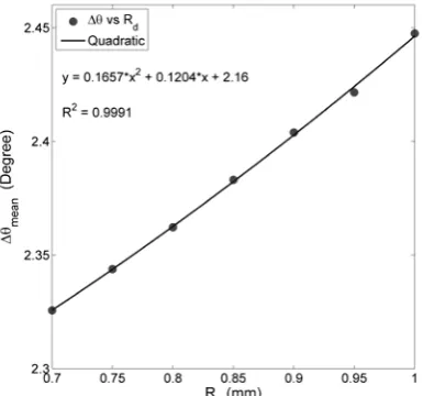
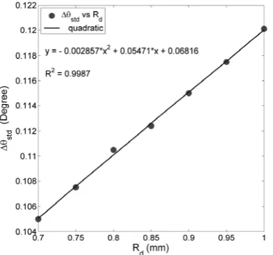
Accuracy evaluation of constructed metamodels for mean and standard deviation of springback is presented in Table II (a) and (b). PRS2 is found to be the most accurate metamodel type for mean value of springback, and KR1 for its standard deviation. For standard deviation, the second most accurate model is found to be PRS2. Both construction and interpretation (mathematical expression is easier and straightforward) of PRS2 models are easier than the other metamodel types. Hence, PRS2 is used for both mean and standard deviation values of springback. The constructed metamodels are found to be accurate when error metrics presented in Table II are compared to presented values in
Table I. The constructed PRS2 models are presented in Figs. 3 and 4. The high R2 values (shown on figures) confirm the
accuracy of PRS2.
Similar to the mean and standard deviation of springback, metamodels are constructed for the mean and standard deviation of the sheet thinning. RBF is found to be the most accurate metamodel type for mean value of sheet thinning, and PRS2 for its standard deviation. As noted earlier, since both creation and interpretation of PRS2 models are easier than the other metamodel types, PRS2 are used for both mean and standard deviation values of sheet thinning. PRS2 models for sheet thinning are constructed similar to Figs. 3 and 4.
TABLEII(A)
ACCURACY EVALUATION VIA CROSS VALIDATION ERROR OF METAMODELS CONSTRUCTED FOR MEAN AND STANDARD DEVIATION VALUE OF SPRINGBACK.THE SMALLEST ERROR METRIC SHOWN IN BOLD FONT.
Mean value of springback Metamodel type RMSE a MAE b MAXEc
PRS2 0.0024 0.0017 0.0048
RBF 0.0053 0.0035 0.0105
KR0 0.0046 0.0027 0.0115
KR1 0.0031 0.0024 0.0060
aRMSE: root mean square error; bMAE: mean absolute error; cMAXE: maximum absolute error
TABLEII(B)
Standard deviation of springback Metamodel type RMSE a MAE b MAXEc
PRS2 0.0003 0.0003 0.0006
RBF 0.0048 0.0032 0.0088
KR0 0.0013 0.0010 0.0029
KR1 0.0002 0.0002 0.0005
[image:4.595.336.529.498.678.2]aRMSE: root mean square error; bMAE: mean absolute error; cMAXE: maximum absolute error
Fig. 4. The change of standard deviation of springback depending on die radius
The equations of constructed PRS2 metamodels are used in the robust optimisation constraint equation (that is, Eq. (13)). The optimum Rd value is calculated as 0.96 mm
which ensures the 5% sheet thinning value with 99% reliability. For this calculated radius value, mean value of sheet thinning is calculated approximately as 4.15%. When MCS (with 10,000 samples) is performed for Rd = 0.96 mm,
the mean value of sheet thinning is calculated approximately as 4.16%. It is another indication that the results obtained from PRS2 are pretty accurate.
The effect of the allowable thinning value on the optimisation results is shown in Table III. It is observed that as the allowable thinning level increases, the optimum die radii reduces, thereby the magnitude as well as the variation of the springback reduces. Notice that the variation is represented by using coefficient of variation, which is the standard deviation over the mean value.
TABLEIII
THE CHANGE OF DIE RADII (RD) AS WELL AS THE MAGNITUDE AND
VARIATION OF SPRINGBACK AND SHEET THINNING WITH RESPECT TO THE ALLOWABLE THINNING LEVEL.
Springback (sb) (°) Sheet thinning (st) (%)
Allowable thinning level (%)
Die radii (Rd)
(mm)
Mean COV a Mean COV a
5 0.96 2.427 0.049 4.160 0.014
10 0.56 2.282 0.043 8.177 0.012
15 0.38 2.250 0.040 12.282 0.010
aCoefficient of variation
V. ASIMPLE SENSITIVITY ANALYSIS
In this section, a simple sensitivity analysis is performed to determine the most influential random variable. The influence of each random variable is evaluated through the following procedure. (1) The value of the random variable of interest is set to μ-3σ and μ+3σ, respectively, while keeping the other random variables at their mean values. (2) The springback values corresponding to these two settings are calculated. (3) The difference between the springback values is a measure of the influence of that random variable. The second column in Table IV shows the springback results when the random variable of interest takes its own
μ-3σ value and the others take their mean values. For example, when yield stress is σY = μ-3σ = 295.87 MPa and
the other random variables take their mean values, springback is calculated as θ = 2.09°. Similarly, the third
column in Table IV shows the springback results when random variable of interest takes the value of μ+3σ while the other random variables take their mean values. The fourth column in Table IV shows the difference between second and third columns. Fifth column shows the normalized values of fourth column. As seen from the fifth column in Table IV, yield stress is found to be the most influential random variable.
TABLEIV
EFFECTS OF RANDOM VARIABLES ON SPRINGBACK.2.42
Variable θμ-3σ (°) θμ+3σ(°) 3 3 (°) Normalized effects
σY 2.09 2.75 0.66 68.1
K 2.38 2.46 0.08 8.3
R 2.38 2.47 0.09 9.2
n 2.43 2.41 0.02 2.1
t 2.48 2.36 0.12 12.3
VI. CONCLUSION
In this study, the magnitude as well as the variation the springback of U-profile sheets made of DP600 dual phase steels were minimized using a robust optimisation methodology. An analytical model was used to predict the sheet springback. The robust optimisation problem was formulated to minimize the mean and the standard deviation of springback subject to a probabilistic constraint on sheet thinning. The reliability level was set to 99% for the probabilistic constraint. The mean and the standard deviation values of springback as well as sheet thinning were computed through Monte Carlo simulations.
If the Monte Carlo simulations were directly integrated into the robust optimisation framework, the computational cost would be very high. To reduce the computational burden, metamodels were constructed for prediction of mean and standard deviation of springback as well as sheet thinning. Four different types of metamodels were utilized, namely second-order polynomial response surface (PRS2), radial-basis functions (RBF) and Kriging (zeroth-order trend model, KR0 and first-order trend model, KR1). PRS2 was found to be the most accurate metamodel type for mean value of springback and the second most accurate metamodel type for its standard deviation. Since both creation and interpretation of PRS2 models are easier than the other metamodel types, PRS2 metamodels are used during optimisation.
Three different sheet thinning levels, namely of 5%, 10% and 15%, were considered and the effects of sheet thinning level on the optimisation results were analyzed. It is found that as the allowable thinning increases the die radius reduces thereby the magnitude and variation of springback reduces.
company resources on reducing uncertainties. For our problem, it is more effective to allocate the resources for tighter quality control measures that can reduce the uncertainty in yield stress.
REFERENCES
[1] T. de Souza, and B. Rolfe, “Multivariate modelling of variability in sheet metal forming”, J Mater Process Technol, vol. 203, no. 1-3, pp.1-12, 2008.
[2] H. Mullerschon, D. Lorenz, and K. Roll, “Reliability based design optimization with LS OPT for a metal forming application” [6. LS DYNA Anwenderforum, Frankenthal, 2007, CIII:1-14]
[3] W. Wang, B. Hou, Z. Lin, and Z. C. Xia, “An Engineering approach to improve the stamping robustness of high strength steels,” J Manuf Sci Eng, vol. 131, no.6, 064501:1-5, 2009.
[4] X. Du, P. K. Venigella, and D. Liu, “Robust mechanism synthesis with random and interval variables”, Mech Mach Theory, vol. 44, no. 7, pp. 1321-1337, 2009.
[5] H. W. Coleman, and W. J. Steele, Experimentation, Validation and Uncertainty Analysis for Engineers. 3rd ed., New York: Wiley, 2009. [6] G. Gantar, and K. Kuzman, “Optimization of stamping processes
aiming at maximal process stability,” J Mater Process Tech, vol. 167, no. 2-3, pp.237–243, 2005.
[7] Z. Dongjuan, Z. Cui, X. Ruan, and Y. Li, “An analytical model for predicting springback and side wall curl of sheet after U-bending”, Comp Mater Sci, vol. 38, no. 4, pp. 707-715, 2007.
[8] I. Ragai, D. Lazim, and J. A. Nemes, “Anisotropy and springback in draw-bending of stainless steel 410: experimental and numerical study”, J Mater Process Tech, vol.166, pp.116–127, 2005.
[9] E. Acar, and M. Rais-Rohani, “Ensemble of metamodels with optimized weight factors,” Struct Multidiscip O, vol. 37, no. 3, pp. 279–94, 2009.
![Fig. 2. The scheme of sheet stretch-bending (Courtesy of [7]), where the Ln is the length of neutral surface, Lm is the arc length of sheet middle surface](https://thumb-us.123doks.com/thumbv2/123dok_us/1292438.658423/2.595.59.272.572.739/stretch-bending-courtesy-length-neutral-surface-length-surface.webp)