Improved SDM-based Robot Navigation
Using Image Processing Techniques
Mateus Mendes
∗ †, A. Paulo Coimbra
∗, and Manuel M. Cris´
ostomo
∗Abstract— Intelligent robot navigation is a broad area of research. Vision-based approaches deserve special attention, for being biologically inspired, in-expensive and powerful. However, problems such as illumination changes, scenario changes and noise are difficult to overcome. In previous work the authors developed algorithms to navigate a robot based on se-quences of visual memories stored into a Sparse Dis-tributed Memory—a kind of associative memory suit-able to work with high-dimensional binary vectors, which also exhibits behaviours in many aspects simi-lar to those of the human brain. This paper analyses the impact of using different image processing tech-niques on the images used: histogram equalisation, contrast normalisation and smoothing using a Gaus-sian filter. The results show that equalisation and smoothing have a positive effect on the performance of the system.
Keywords: Robot Navigation, View-based Navigation, Image Processing, SDM, Sparse Distributed Memory
1
Introduction
Many different approaches have been tried to localise and navigate robots in a safe and robust way. Some of those approaches can only be used in structured environments, since they are based on the recognition of artificial land-marks, beacons or similar strategies that improve the ac-curacy of the system but require special conditions [1]. More generic strategies that work in unstructured envi-ronments include mapping and localisation using laser range finders, sonars or cameras.
Vision-based approaches are biologically inspired, since humans use mostly vision for localisation [2]. The sen-sors required are inexpensive, but the processing power needed is huge. Every single image is usually described by hundreds or thousands of pixels, and every path that the robot learns is described by tens, hundreds or thousands of images. The use of cognitive information, in which the raw images are replaced by formal descriptions of the contents of the images, may solve part of the problem. But that is still an open area of research.
∗ISR - Institute of Systems and Robotics, Dept. of Electrical and
Computer Engineering, University of Coimbra, Portugal. E-mail: [email protected], [email protected]. †ESTGOH, Polytechnic
In-stitute of Coimbra, Portugal. E-mail: [email protected].
The images alone are a means for instantaneous local-isation. View-based navigation is almost always based on the same idea: during a supervised learning stage the robot learns a sequence of views that, if followed with minimum drift, will lead it to a target location. By fol-lowing the sequence of commands, possibly correcting the small drifts that may occur, the robot is later able to fol-low the learnt path autonomously [3]. To a great extent, this view-sequence based approach is similar to the way the human brain works [4, 5].
In previous work the authors presented a system to navi-gate a robot using images stored into a Sparse Distributed Memory (SDM) [6]. The SDM is a kind of associa-tive memory based on the properties of high-dimensional boolean spaces, and thus suitable to work with large bi-nary vectors such as raw images [4]. The present pa-per describes expa-periments using different image process-ing techniques, in order to make the system more robust to illumination changes and image noise.
Section 2 explains navigation based on view sequences. Section 3 briefly describes the SDM. In Section 4 the experimental platform is presented. Section 5 describes the image processing techniques used. Section 6 shows and discusses the results obtained, and Section 7 draws some conclusions and opens perspectives of future work.
2
Navigation using view sequences
The approach followed to navigate the robot is based on using visual memories stored into a SDM, as described in [6]. It requires a supervised learning stage, in which the robot is manually guided. While being guided, the robot memorises a sequence of views automatically. It stores a sequence of views for each path. Images that are very similar to previously stored images are discarded, because they would, with high probability, not add any relevant information to the known information.
the horizontal distance between them in order to infer
how far it is from the correct path. The technique is described in more detail in [6].
3
Sparse Distributed Memory
The Sparse Distributed Memory is an associative mem-ory model proposed by Kanerva in the 1980s [4]. It is suitable to work with high-dimensional binary vectors. Kanerva shows that the SDM exhibits the properties of large boolean spaces, which are, to a great extent, sim-ilar to that of the human cerebellum. The SDM natu-rally implements behaviours such as tolerance to noise, operation with incomplete data, parallel processing and
knowing that one knows.
In the proposed approach, an image is regarded as a high-dimensional vector, and the SDM is used simultane-ously as a sophisticated storage and retrieval mechanism and a pattern recognition tool. For space constraints the original SDM model is not described in the present pa-per. A description can be found, for example, in [7]. In the present work, a model that we call “auto-associative arithmetic” is used, as exemplified in Figure 1. The main modules of the SDM are an array of addresses and an array of data vectors. It is even acceptable an auto-associative version, in which the same array is used si-multaneously as addresses and data, as long as datum ζ is only stored at locationζ. The auto-associative memory needs about one half of the storage space.
Every input address will activate all the memory ad-dresses that are within a predefined activation ra-dius. Different methods can be used for computing the distance—the present implementation uses the sum of the absolute differences. In Figure 1 the example address vector<90,95>will activate address<100,106> (dis-tance 21) and address<110,90>(distance 25).
Reading from the memory is done by averaging the in-teger values columnwise. Learning is achieved updating each byte value using the equation:
hk
t =hkt−1+α·(x
k−hk
t−1), α∈R∧0≤α≤1 (1)
In the equation, hk
t is the kth number of the memory location, at time t, xk is the corresponding number in the input vector x and α is the learning rate. In the present implementation α was set to 1, enforcing one-shot learning.
[image:2.595.373.485.72.149.2]The memory locations are managed using the Ran-domised Reallocation (RR) algorithm [8]. Using the RR, the system starts with an empty memory and allocates new locations when there is a new datum which cannot be stored into enough existing locations. The new loca-tions are placed randomly in the neighbourhood of the new datum address.
[image:2.595.370.485.181.284.2]Figure 1: Auto-associative arithmetic SDM.
Figure 2: Robot used.
4
Experimental platform
The robot used is a Surveyor1
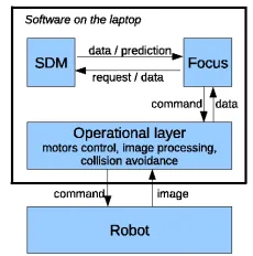
SRV-1 (Figure 2). Among other features, it has a built in digital video camera and a 802.15.4 radio communication module. It is controlled in real time from a laptop. The overall software architecture is as shown in Figure 3. It contains three basic modules: i) the SDM, where the information is stored; ii) the Focus (following Kanerva’s terminology), where the navigation algorithms are run; and iii) an operational layer, respon-sible for interfacing the hardware and some tasks such as motor control, collision avoidance and image processing.
For vision-based navigation, the vectors stored in the SDM consist of arrays of bytes, as summarised in Equa-tion 2:
xi=< imi, seq id, i, timestamp, motion > (2)
In vectorxi,imi is the imagei, in PGM (Portable Grey Map) format and 80×64 resolution. In PGM images, ev-ery pixel is represented by an 8-bit integer: 0 is black,
1http://www.surveyor.com.
[image:2.595.369.484.615.731.2]255 is white. seq idis an auto-incremented, 4-byte inte-ger, unique for each sequence. It is used to identify which sequence the vector belongs to. iis an auto-incremented, 4-byte integer, unique for every vector in the sequence, used to quickly identify every image in the sequence. timestampis a 4-byte integer, storing Unix timestamp. It is not being used so far for navigation purposes. motion is a single character, identifying the type of movement the robot performed after the image was grabbed. The image alone uses 5120 bytes. The overhead information comprises 13 additional bytes. Hence, the input vector contains 5133 bytes.
5
Image processing
Three different image processing techniques have been tried: contrast normalisation, equalisation and smooth-ing.
5.1
Contrast enhancement
The quality of images as grabbed directly from the cam-era depends a lot on ambient illumination. Dim light produces dark images with little contrast, while good il-lumination provides images with better contrast. Under dim light the pixel values will tend towards 0, the black pixel. Under strong light the values will move towards the other end of the interval: 255, the white pixel. The dif-ference between two such images may eventually lead the system to consider them as two different pictures, even if they correspond to the same view. The problem may be minimised using techniques to adjust the distribution of the pixel values, enhancing the contrast of the images.
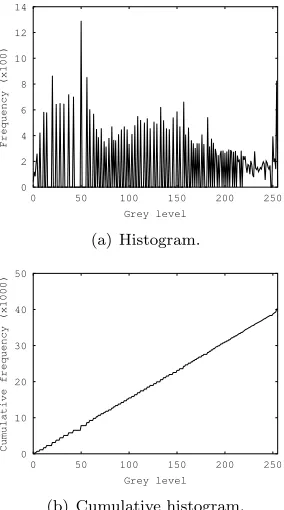
Figure 4 shows an image captured under dim light, and the corresponding frequency distribution of the pixel val-ues and cumulative histograms. As shown, the image is very dark—it is rich in brightness intensities below 150 and contains almost no values above that level. The grey levels with higher frequencies are in general below 50. The cumulative histogram is a curve which rises very fast until 100 and a horizontal line above 150.
5.1.1 Contrast stretching
Contrast stretching (also called contrast normalisation) is a method that consists in applying a linear function to the image, in order to improve its contrast. The in-tensities of an image with poor contrast, such as the test image shown in Figure 4(a), do not extend through the full range of available pixel values. In the case of the test image they all actually fall in the range [7, 178]. Ap-plying a linear transform to the image it is possible to stretch the intensity levels so that they occupy all the range [0, 255], resulting in an image with improved con-trast. Mathematically, the technique is simply a function
that maps one interval into another interval:
f : [a, b]−→[c, d] (3)
In 3, a and b are the minimum and maximum intensity levels found in the image, and canddare the minimum and maximum intensity levels that can be used. The value of each pixel Pin is then reassigned into Pout, ac-cording to Equation 4:
Pout =c+ (Pin−a)
d
−c b−a
(4)
Figure 5 shows the result of applying the contrast-stretching transform to the image. As shown, both ends of the the histogram were stretched, so that it occupies all the range [0, 255]. There is at least one pixel with inten-sity 0, and there is also at least one pixel with inteninten-sity 255.
5.1.2 Histogram equalisation
Histogram equalisation is a technique to manipulate im-ages based on the analysis of the corresponding his-tograms. The method consists in taking the original cu-mulative histogram of the original image, normalise it to-wards 255 (or the maximum intensity value that can be found in the image), and then use it as a mapping func-tion to the original image, thus achieving a uniform his-togram after the transform. The uniform hishis-togram ob-tained will correspond to a brightness distribution where all the values should be equally probable. Due to the discrete nature of the digital images, the result is usually just an approximation. Nonetheless, the technique re-sults in a significant improvement of the original images, as shown in Figure 6.
The procedure is formalised as follows. First, let’s con-sider an imagex, ofL different grey levels andn pixels. Letni be the number of occurrences of grey leveli in the image. The probability of occurrence of a pixel of leveli in the image is given by equation:
px(i) =p(x=i) =ni
n, i∈0, ..., L (5)
Probabilitypx(i) is, indeed, the same as the grey level’s frequency value in the histogram, once it is normalised into the interval [0, 1]. The cumulative probability dis-tribution function of p also coincides with the image’s normalised cumulative histogram:
c(i) = i
X
j=0
px(j), i∈0, ..., L (6)
(a) Original image, as captured under dim light.
0 1 2 3 4 5 6 7
0 50 100 150 200 250
Frequency (x100)
Grey level
(b) Histogram.
0 5 10 15 20 25
0 50 100 150 200 250
Cumulative frequency (x1000)
Grey level
[image:4.595.79.516.73.205.2](c) Cumulative histogram.
Figure 4: Image captured under dim light, and corresponding frequency and cumulative histograms.
0 2 4 6 8 10 12 14
0 50 100 150 200 250
Frequency (x100)
Grey level
(a) Histogram.
0 10 20 30 40 50
0 50 100 150 200 250
Cumulative frequency (x1000)
Grey level
[image:4.595.149.446.249.375.2](b) Cumulative histogram.
Figure 5: Frequency and cumulative histograms of the image after contrast stretching.
0 2 4 6 8 10 12 14
0 50 100 150 200 250
Frequency (x100)
Grey level
(a) Histogram.
0 10 20 30 40 50
0 50 100 150 200 250
Cumulative frequency (x1000)
Grey level
(b) Cumulative histogram.
Figure 6: Frequency and cumulative histograms of the image after histogram equalisation.
the value range. That is, if it is used the transformation of Equation 7 to map every pixel value in the image from xto y, the output image will exhibit a linear histogram in the co-domain [0, 1].
yi =c(i)·xi, i∈0, ..., L (7)
To get the image back into the original [0, L] interval, it is necessary to apply a linear transform to stretch the co-domain:
y′
i=yi·L (8)
For real time processing, it is possible to merge equations 6, 7 and 8 together. That way it is possible to skip the prior normalisation of the cumulative histogram into the interval [0, 1] and perform all the operations with a single loop to process all the image (providing the cumulative histogram has already been computed) [9], as shown in Algorithm 1.
Algorithm 1:Histogram equalisation
begin
alpha←−L/numP ixels;
foreach pixel do
y←−C(x)∗alpha;
[image:4.595.97.239.441.696.2](a) Original. (b) Normalised.
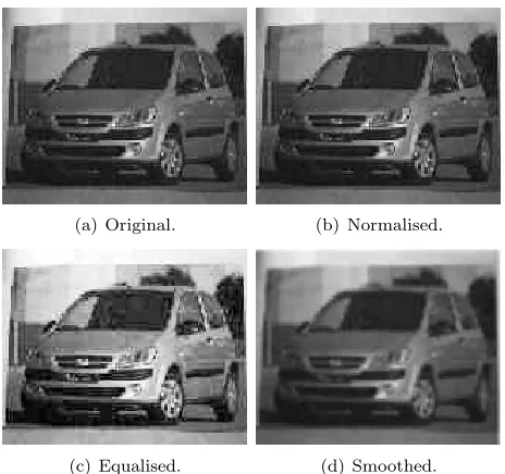
[image:5.595.54.286.69.287.2](c) Equalised. (d) Smoothed.
Figure 7: Comparison of the original, normalised, equalised and smoothed images.
In Algorithm 1,numP ixelsis the total number of pixels in the image, andC(x) the cumulative frequency of grey levelx.
5.2
Smoothing
Gaussian filters are often used in image processing as a way to reduce noise levels. The final image is blurred, and the contours are smoother than they were in the original image. The process consists of running through the image a filter in which each pixel is replaced by a weighted aver-age of the neighbouring pixels, where the nearest neigh-bours contribute more than the farthest neighneigh-bours, ac-cording to the Gaussian function. For an image, a two dimensions Gaussian must be applied, as shown in Equa-tion 9.
G(x, y) = 1 2πσ2e
−x2 +y
2
2σ2 (9)
In the formula,σis the standard deviation of the Gaus-sian distribution. A largeσwill give more importance to farther pixels, while a smallσ gives more importance to the nearest pixels. In practise, pixels outside the radius 3σare usually ignored, for their contribution to the final value is negligible.
In the present work, the Gaussian filter was applied using OpenCV library2
. The standard deviation was computed automatically, but only the contributions of the immedi-ate neighbours were used.
Figure 7 shows the original image, a contrast stretched image, an equalised image and a smoothed image. Ob-viously, the same image can be subject to different
pro-2http://opencv.willowgarage.com/wiki/ (last checked
2012.02.27).
cessing methods. For example, it makes sense to smooth an image and then equalise. It makes no sense to equalise and contrast stretch, since both methods intend to achieve the same goal, and contrast stretch will have no effect on an equalised image.
6
Experiments and results
To assess the performance of the system, the concept of “Momentary Localisation Error” (MLE) was defined. A MLE is counted when the robot, in the autonomous run mode, retrieves imageimj−i after retrieving imageimj, fori, j >0. When that happens, it means that one of the predictions was wrong, because the robot is not expected to get back in the sequence. Most MLEs are not fatal: a wrong prediction may still lead to a correct robot move; a wrong move may not lead the robot to get lost; and the effect of a wrong move may be neutralised right away by the drift correction algorithm. Nonetheless, most MLEs may cause delays to the robot, if they make it perform a wrong move.
6.1
Experiments
The experiments performed consisted in teaching the robot a path described by about 100 images. Later, the robot was made to follow the same path again, under different illumination levels and applying different image processing techniques.
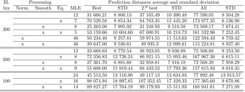
Table 1 summarises the results of one experiment, in which the robot was following a path described by 120 images in a testbed. The path was taught with ambient illumination of about 300 Lux. The first column of the table states the approximate illumination level during the autonomous runs. Columns 2–4 identify which process-ing methods were applied. Column 5 shows the number of MLEs that have been counted for each experiment. It should be noted that the step of the robot during the au-tonomous run is about 1/4 of the learning step size, hence 12 MLEs actually represent prediction errors in about 2.5% of the predictions. Column 6 is the average of the best similarity measures, measured between the robot’s
current view and the pool of images in the SDM. Column 7 is the corresponding standard deviation. Columns 8 is the average distance to the second best prediction. Com-paring columns 6 and 7 it is possible to have an idea of how successful the system is in separating the best pre-diction from the second best. Column 9 is the standard deviation of the 8th column. Column 10 is the average distance between the current image and the pool of im-ages in the SDM.
6.2
Discussion
Table 1: Results with path described by 120 images. Suppressed lines on lower illumination levels mean the robot did not finish the path.
Ill. Processing Prediction distances average and standard deviation lux Norm. Smooth Eq. MLE Best STD 2.ºbest STD All STD
300
12 31 666.21 8 800.13 37 165.49 10 390.48 77 590.05 8 504.28 x 7 70 529.58 9 854.34 84 783.35 15 445.20 173 977.35 6 136.90 x 8 25 263.00 7 995.92 31 248.93 9 510.58 73 569.17 7 674.41 x x 5 53 159.66 10 604.60 67 000.91 16 218.73 161 532.96 7 252.45 x 46 50 234.40 9 257.81 59 974.55 11 513.63 122 594.43 8 759.42 x x 46 39 647.00 9 530.61 49 935.3 12 098.61 115 224.81 8 927.40
200
12 33 668.63 8 770.54 38 923.05 9 030.89 75 506.68 9 253.50 x 8 72 356.83 12 726.24 86 921.15 15 093.46 167 967.36 6 615.11 x 8 27 361.70 6 881.68 32 958.81 7 816.18 72 568.28 7 958.29 x x 9 55 608.00 15 919.44 68 433.52 17 793.36 157 815.93 8 018.35
100
24 45 513.50 13 110.90 49 117.13 13 634.93 77 992.48 13 913.57 x 16 98 074.94 18 997.85 107 352.45 17 429.33 177 365.60 9 670.86 x x 14 89 827.27 17 764.19 99 179.93 15 511.93 168 941.61 7 271.88
also increases. When the illumination level is reduced, us-ing contrast stretched images the robot does not complete the path. Equalisation has a very large impact on the av-erage distances. That happens because the pixel values are stretched over all the domain for histogram equalisa-tion. But in this case the processing has a positive impact on the number of localisation errors. And that effect is even more pronounced when the illumination is reduced. Using equalised images the robot is always able to com-plete the path. Smoothing the images using the Gaussian filter greatly reduces the average distances. That is an expected result, since the pixel values are approximated to the values of the neighbouring pixels. The performance of the system is excellent with smoothing alone, except when the illumination is very faint. In that case equali-sation is required for the robot to successfully complete the path.
In summary, the results show that noise reduction through the use of a Gaussian filter and histogram equal-isation largely contribute to robust navigation. They re-duce the number of momentary localisation errors, thus improving the speed and accuracy of the process, and help the robot finish the path even under dim light.
7
Conclusions
Intelligent robot navigation based on visual memories is a long sought goal. However, there are many problems to be solved, such as the presence of noise in the images and illumination changes. The approach followed in the present work relies on memories stored into a SDM. The performance of the system is improved by processing the images using a Gaussian filter and histogram equalisa-tion. Contrast normalisation usually produces bad re-sults. Future research will be done in order to identify relevant objects or features in the images. The vectors
stored into the SDM will contain feature information, leading the way to work at a cognitive level. That should improve the performance of the system and possibly de-crease memory storage and/or processing time needs.
References
[1] Christopher Rasmussen and Gregory D. Hager. Robot navigation using image sequences. In Proc. 13th
Na-tional Conf. on AI, pages 938–943. AAAI Press, 1996. [2] Steven Johnson.Mind wide open. Scribner, New York,
2004.
[3] Yoshio Matsumoto, Masayuki Inaba, and Hirochika Inoue. View-based approach to robot navigation. In
Proc. of IEEE/RSJ IROS 2000, 2000.
[4] Pentti Kanerva. Sparse Distributed Memory. MIT Press, Cambridge, 1988.
[5] Jeff Hawkins and Sandra Blakeslee. On Intelligence. Times Books, New York, 2004.
[6] Mateus Mendes, Manuel M. Cris´ostomo, and A. Paulo Coimbra. Robot navigation using a sparse distributed memory. InProc. of IEEE Int. Conf. on Robotics and Automation, Pasadena, California, USA, May 2008. [7] Mateus Mendes, Manuel M. Cris´ostomo, and A. Paulo
Coimbra. Assessing a sparse distributed memory us-ing different encodus-ing methods. In Proc. of World Congress on Engineering, London, UK, July 2009. [8] Bohdana Ratitch and Doina Precup. Sparse
dis-tributed memories for on-line value-based reinforce-ment learning. InECML, 2004.