The LMU System for the CoNLL-SIGMORPHON 2017 Shared Task on
Universal Morphological Reinflection
Katharina Kann and Hinrich Sch¨utze CIS
LMU Munich, Germany [email protected]
Abstract
We present the LMU system for the CoNLL-SIGMORPHON 2017 shared task on universal morphological reinflection, which consists of several subtasks, all con-cerned with producing an inflected form of a paradigm in different settings. Our solution is based on a neural sequence-to-sequence model, extended by prepro-cessing and data augmentation methods. Additionally, we develop a new algorithm for selecting the most suitable source form in the case of multi-source input, outper-forming the baseline by 5.7% on aver-age over all languaver-ages and settings. Fi-nally, we propose a fine-tuning approach for the multi-source setting, and combine this with the source form detection, in-creasing accuracy by a further4.6%on
av-erage.
1 Introduction
Many of the world’s languages have a rich mor-phology, i.e., make use of surface variations of lemmata in order to express certain properties, like the tense or mood of a verb. This makes a variety of natural language processing tasks more chal-lenging, as it increases the number of words in a language drastically; a problem morphological analysis and generation help to mitigate. How-ever, a big issue when developing methods for morphological processing is that for many mor-phologically rich languages, there are only few or no relevant training data available, making it impossible to train state-of-the-art machine learn-ing models (e.g., (Faruqui et al., 2016;Kann and Sch¨utze, 2016b; Aharoni et al., 2016; Zhou and Neubig, 2017)). This is the motivation for the CoNLL-SIGMORPHON-2017 shared task on
uni-versal morphological reinflection (Cotterell et al., 2017a), which animates the development of sys-tems for as many as 52 different languages in 6 different low-resource settings for morphological reinflection: to generate an inflected form, given a target morphological tag and either the lemma (task 1) or a partial paradigm (task 2). An exam-ple is
(use, V;3;SG;PRS)7→uses
In this paper, we describe the LMU system for the shared task. Since it depends on the language and the amount of resources available for training which method performs best, our approach con-sists of a modular system. For most medium- and high-resource, as well as some low-resource set-tings, we make use of the state-of-the-art encoder-decoder (Cho et al.,2014a;Sutskever et al.,2014; Bahdanau et al.,2015) network MED (Kann and Sch¨utze,2016b), while extending the training data in several ways. Whenever the given data are not sufficient, we make use of the baseline system, which can be trained on fewer instances.
While we submit solutions for every language and setting, our main focus is on task 2 of the shared task and the main contributions of this pa-per correspondingly address a multi-source input setting: (i) We develop CIS (”choice of important sources”), a novel algorithm for selecting the most appropriate source form for a target tag from a partially given paradigm, which is based on edit trees (Chrupała, 2008). (ii) We propose to cast the task of multi-source morphological reinflec-tion as a domain adaptareinflec-tion problem. By fine-tuning on forms from a partial paradigm, we im-prove the performance of a neural sequence-to-sequence model for most shared task languages.
Our final methods, averaged over languages, outperform the official baseline by7.0%,18.5%,
and 16.5% for task 1 and 8.7%, 10.1%, and
10.3%for task 2 for the low-, medium-, and high-resource settings, respectively.
Furthermore, our submitted sytem—a combina-tion of our methods with the baseline system— surpasses the baseline’s accuracy on test for both tasks as well as all languages and settings. Differ-ences in performance are between 8.69% (task 1 low) and17.94%(task 1 medium).
2 Morphological Reinflection
The paradigm of a lemmawlis a set of tuples of inflected formsfkand tagstkdescribing the prop-erties of the inflected word, which we formally de-note as:
π(wl) =
n
fk[wl], tko
tk∈T(wl)
(1)
withT(wl)being the set of possible tags forwl. An example is the following paradigm of the Spanish lemmaso˜nar:
π(so˜nar) =n sue˜no,1SgPresInd, . . . , so˜naran,3PlPastSbjo
The shared task has two subtasks: task 1 con-sists of predicting a certain formfi[wl], given the lemmawl and the target tag ti. Fortask 2, one or more source forms are given for each lemma (multi-source input). Thus, additional information about the way a lemma is inflected is known and can be leveraged.
3 Preprocessing Methods
We apply the following preprocessing methods.
String preprocessing. We determine for each
language if it is predominantly prefixing or suf-fixing, using the same algorithm as the shared task baseline system (Cotterell et al.,2017a). For pre-fixing languages, we invert all words. An example for the prefixing language Navajo is:
chid´ı→´ıdihc
New character handling. The source and target
vocabularies for the languages are constructed us-ing the respective trainus-ing and development sets. Therefore, out-of-vocabulary symbols can appear in the test sets, resulting in symbols the model has no information about. In order to address this, we substitute such characters by a specialNEW sym-bol and train the model on it by including it in the additional training samples we create, cf. §4.
In the output,NEWis substituted back by the new characters in the input in order of appearance. An example from the German development data is:
Phlo¨em→PhloNEWm
Tag extension. Explicit information is usually
handled better by machine learning methods than implicit information. Therefore, we search for op-tional subtag slots, in contrast to those that are al-ways occupied by some value, e.g., an optional
negationsubtag, in contrast to the part-of-speech subtag which, for most languages, is always ei-ther Verb, Noun or Adjective, but never empty. For all optional subtags, we artificially introduce a negated form.
4 Training Data Augmentation Methods
Additional source-target form pairs. We
col-lect all forms belonging to the same lemma. We then add additional samples by constructing source-target combinations for other sources than the lemma, using the members of each paradigm. For the two samples lemmai → word1 and lemmai→word2we can introduce the new
sam-plesword1→word2andword2→word1.1
Autoencoding samples. We further create
sam-ples for a sequence autoencoding task, i.e., we add mappings of words to themselves, with a special copy tagA. No morphological tags are given. This is a way to multi-task train on autoencoding the input string and reinflection, as we maximize the joint log-likelihood
L(θ) = X (wl,ts,tt)∈T
logpθ(ft(wl)|e(fs(wl), tt))
(2)
+ X
w∈W
logpθ(w|e(w))
for the training data T, source and target tagsts and tt, a lemma wl and an encoding function e depending onθ, as well as a set of stringsW. We apply two variants: autoencoding the lemmata and forms from the original training set, or using ran-domstrings for this. Random strings are produced in the following way. We first construct all pos-sible bigrams B from the vocabulary of the lan-guage. We then combine those with a random se-quence of charactersrof a random length between
1The respective source and target tags are part of the input,
1 and 4 in the following way:b1+b2+r+b3+b4
forbi ∈ B. Constructing random strings like this has the positive side-effect that we can add aNEW to the vocabulary.
Rule-based data generation. We imitate a
rule-based system by, given a source form and a tar-get form, defining the prefix (resp. suffix) of a word as the word minus the longest common suf-fix (resp. presuf-fix). We then create an additional training example by generating a random strings and prepending (resp. appending) source and tar-get prefixes (resp. suffixes) tos. For example, in German, we can find the following rule for the 2nd person singular form:
*en→*st
From this we can create additional training in-stances like the following.
(jfgdgfen, V;2;SG;PRS)7→jfgdgfst (Ahggen, V;2;SG;PRS)7→Ahggst
We apply this procedure to all pairs of a source and a target tag that appear less thanttimes in train for a certain thresholdt.
5 System Architecture
We apply the encoder-decoder network MED (Kann and Sch¨utze, 2016a), due to its success in last year’s edition of the shared task (Cotterell et al., 2016). While we extend it by new train-ing data augmentation methods and, for task 2, the additional algorithms described below, we do not make changes to the model’s architecture. We will shortly describe MED and the shared task baseline system in this section.
5.1 MED
Encoder. The format of the input of the encoder
is the same as in (Kann and Sch¨utze,2016a), but with a small modification to be able to handle un-labeled data: Given the set of morphological sub-tags M that each target tag is composed of (e.g., the tag1SgPresIndcontains the subtags1,Sg,Pres
andInd), and the alphabetΣof the language of
ap-plication, our input is of the form(A|M∗) Σ∗, i.e., it consists ofeither a sequence of subtags orthe symbolAsignaling that the input is not annotated and should be autoencoded, and (in both cases) the character sequence of the input word. All parts of the input are represented by embeddings.
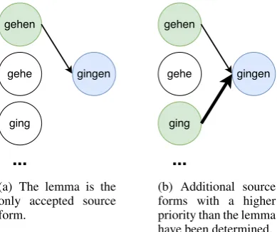
(a) The lemma is the only accepted source form.
[image:3.595.320.515.66.229.2](b) Additional source forms with a higher priority than the lemma have been determined. Figure 1: Comparison of the traditional view (left) and the re-sult of CIS (right). Possible source forms in green, the target form in blue. Thickness of the arrows represents priorities of source forms. Most forms of the paradigm have been omitted because of space limitations.
We encode the input x = x1, x2, . . . , xTx
us-ing a bidirectional gated recurrent neural network (GRU) (Cho et al., 2014b). We then concatenate the forward and backward hidden states to obtain the inputhifor the decoder.
Decoder. The decoder is a uni-directional
attention-based GRU, defining a probability dis-tribution over strings inΣ∗:
p(y |x) =
Ty
Y
t=1
p(yt|y1, . . . , yt−1, st, ct),
with st being the decoder hidden state for time
t andct being a context vector, calculated using the encoder hidden states together with attention weights. A detailed description of the encoder-decoder model can be found in (Bahdanau et al., 2015).
5.2 Baseline System
Figure 2: Edit tree for the transformation from abgesagt
“canceled” toabsagen“to cancel”. Each node contains the length of the parts before and after the respective LCS, e.g., the leftmost node contains the length of the parts before and after the LCS ofabgeandab. The prefixsubindicates that the node is a substitution operation.
6 Choice of Important Sources
As ourchoice of important sources (CIS)
algo-rithm is based strongly on edit trees (Chrupała,
2008), we will introduce them first.
Edit trees. An edit treee(σ, τ)is a way to
spec-ify a transformation between a source stringσand a target stringτ(Chrupała,2008). It is constructed by first determining the longest common substring (LCS) (Gusfield,1997) ofσandτ and then mod-eling the prefix and suffix pairs of the LCS recur-sively. In the case of an empty LCS,e(σ, τ)
corre-sponds to the substitution operation that replaces σwithτ. Figure2shows an example.
CIS. The entire task of paradigm completion is built upon the notion that the members of a paradigm are not independent. However, for many languages, some slots of a paradigm are more dependent on each other: For example, gehen,
geheandging are all forms of the same German paradigm, but when aiming to produce the 3rd per-son plural past tense formgingen, the task is easier when starting from the (more similar) formging. In fact, in many cases, the entire paradigm is com-pletely deterministicwhen the right paradigm slots are known. A set of forms that determines all other inflected forms is calledprincipal parts.
(Cotterell et al., 2017b) use this property of morphologically rich languages to induce topolo-gies in order to jointly decode entire paradigms and to thus make use of all known forms. However, they suppose to be able to compute and use good estimates for the probabilities p(fi(wl)|fj(wl))for source form fj(wl) and tar-get form fi(wl), since they use at least 632 en-tire paradigms per part of speech and language for training. Using a minimum spanning tree, they ap-proximate a solution to the maximum-a-posteriori
Figure 3: Overview of a fine-tuning setup. In our case, “in-domain” refers to the partial paradigm to be completed; “out-of-domain” refers to all other paradigms.
(MAP) inference problem.
In order to be able to apply our approach to low-resource settings, we focus instead on find-ing the best source form for each target form in a language, and CIS works as follows. We cal-culate edit trees for each pair(fj(wl), fi(wl))for each lemmawlin the training data. We then count the number of different edit trees for each pair of source and target tag(tj, ti) and build an impor-tance list for each tag ti, giving higher priorities to source tags with lower counts. The intuition be-hind this is that the fewer different edit trees ap-pear in the training set, the more deterministic the paradigm slotiis, given a certain source slotj.
At test time, we find the form from the given slots of the paradigm which has the highest impor-tance score, and use it to generate the target form. Note that, as the lemma is always given, there will never be a need to use a worse source form than the lemma.
7 Fine-Tuning for Multi-Source Input For sequence-to-sequence models for neural ma-chine translation, it has been shown that special-ized models for a certain domain are able to ob-tain better performances than general ones ( Lu-ong and Manning, 2015). One way to perform such adomain adaptationis fine-tuning: a general model, which has been trained on out-of-domain data, is further trained on (newly) available in-domain data, cf. Figure 3. This brings the con-ditional probabilityp(y1, ..., ym|x1, ..., xn)for an output sequence (y1, ..., ym) given an input se-quence (x1, ..., xn) closer to the target distribu-tion.
Here, we propose to improve multi-source mor-phological reinflection by treating each paradigm as a separate domain and performing “domain adaptation” everytime a new paradigm should be completed by the model.
[image:4.595.123.239.66.142.2]n≤1.5 1.5< n <10 10≤n
danish arabic albanian
english bengali armenian
norwegian-bokmal bulgarian basque norwegian-nynorsk czech catalan
dutch haida
estonian hindi faroese italian finnish khaling french persian georgian portuguese
german quechua hebrew sorani hungarian spanish
icelandic turkish
irish urdu
kurmanji welsh latin
latvian lithuanian lower-sorbian
macedonian navajo northern-sami
polish romanian
russian scottish-gaelic serbo-croatian
[image:5.595.80.283.61.396.2]slovak slovene swedish ukrainian
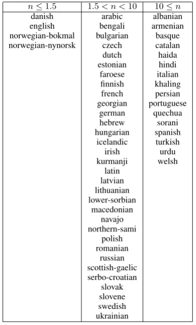
Table 1: Average amount n of sources given per paradigm, for the development set.
each setting and language), trained on all avail-able training examples. The original training data corresponds to out-of-domain data in a domain adaptation setting. At test time, we construct for each partial paradigmPknownall possible training examples in the way described in the paragraphs about additional source-target form pairs and au-toencoding in §4. Thus, for|Pknown| = n, we end up with (up to) n∗(n−1) +Na in-domain samples for fine-tuning whereNais the number of autoencoding training samples. We then for each partial paradigm fine-tune the original base model on all examples constructed from Pknown, which match thein-domain data for domain adaptation. Thus, we end up with a different fine-tuned model for each partial paradigm in the test set.
Our method is expected to perform best in a set-ting in which many forms of each paradigm are given as input, e.g., whennis big. Table1 indi-cates for which language we would therefore ex-pect could performance.
8 Experiments
8.1 Systems
Task1. For task 1, we apply MED*: MED in
combination with all preprocessing methods men-tioned in §3 and the following data augmenta-tions. We create additional source-target form pairs where possible and create autoencoding sam-ples, random ones as well as from the original data. Further, we create 5 additional rule-based samples for each existing sample of all source-target tag combinations that appear less thant = 10times in the training set for a language.
We employ ensembles of 5 MED* models, which are trained for 90 (low and medium) or 45 (high) epochs. Ensembling is done by majority voting.
Task2. We again apply MED*. However, for
task 2 we do not create rule-based samples.2
Mod-els for the low-resource, medium-resource and high-resource settings are trained for 45, 30 and 20 epochs, respectively. For task 2, we do not use ensembling.
At test time, we preprocess each newly incom-ing paradigm in the same way as the trainincom-ing data, except for the creation of random copy samples. We then fine-tune the base model for each new paradigm according to§7for 25 additional epochs. Additionally, we choose the best source form for each required target tag and predict each inflected form for this input (MED*+FT+CIS).
The limited amount of data makes it impos-sible to obtain competitive performance using MED* for some languages and settings (espe-cially for languages with only few given slots per paradigm), even after applying all data augmen-tation methods described above. Thus, we apply the baseline model for those cases, but combine it with CIS (cf. §6) to improve its performance
(BL+CIS). We do not apply preprocessing or data
augmentation methods for BL, as they would not influence its performance.
Shared task submission. The best approach
de-pends on both the language and the setting. Thus, our final submission for each case is obtained by either BL, BL+CIS, the MED* ensemble, or MED*+FT+CIS, selected using the accuracy on the development set.
2Using rule-based examples for training leads to worse
low medium high
BL MED* MED* (ENS) BL MED* MED* (ENS) BL MED* MED* (ENS) albanian 0.216 0.102 0.129 0.661 0.849 0.878 0.781 0.966 0.975
arabic 0.215 0.237 0.298 0.400 0.804 0.842 0.477 0.930 0.952
armenian 0.378 0.444 0.488 0.766 0.897 0.914 0.891 0.972 0.975 bulgarian 0.331 0.437 0.480 0.750 0.814 0.837 0.900 0.969 0.974 catalan 0.552 0.560 0.598 0.832 0.903 0.930 0.942 0.981 0.983
czech 0.408 0.318 0.341 0.807 0.815 0.856 0.904 0.927 0.937
danish 0.598 0.636 0.654 0.781 0.830 0.845 0.891 0.934 0.960
dutch 0.537 0.500 0.521 0.717 0.828 0.862 0.868 0.968 0.971
english 0.762 0.831 0.852 0.902 0.928 0.940 0.950 0.964 0.968 faroese 0.307 0.347 0.386 0.587 0.595 0.672 0.747 0.817 0.867 finnish 0.162 0.120 0.147 0.425 0.682 0.754 0.785 0.939 0.954
french 0.630 0.579 0.635 0.761 0.789 0.820 0.836 0.889 0.914
georgian 0.712 0.802 0.845 0.900 0.925 0.928 0.940 0.991 0.995
german 0.537 0.541 0.593 0.715 0.772 0.800 0.812 0.894 0.912
hebrew 0.279 0.335 0.366 0.400 0.798 0.831 0.558 0.987 0.991
hindi 0.310 0.781 0.782 0.866 0.964 0.974 0.940 1.000 1.000
hungarian 0.172 0.300 0.346 0.417 0.708 0.763 0.711 0.856 0.874 icelandic 0.342 0.341 0.364 0.614 0.647 0.689 0.761 0.873 0.913 italian 0.449 0.392 0.467 0.738 0.920 0.927 0.799 0.978 0.974 latvian 0.621 0.483 0.536 0.851 0.834 0.861 0.910 0.965 0.977 lower-sorbian 0.343 0.451 0.488 0.705 0.788 0.817 0.860 0.966 0.973 macedonian 0.500 0.577 0.664 0.823 0.901 0.913 0.919 0.957 0.964
navajo 0.184 0.166 0.198 0.313 0.415 0.460 0.383 0.838 0.897
northern-sami 0.154 0.136 0.174 0.357 0.639 0.711 0.611 0.954 0.968 norwegian-nynorsk 0.508 0.489 0.559 0.633 0.671 0.687 0.783 0.883 0.923 persian 0.273 0.405 0.457 0.654 0.892 0.913 0.776 0.999 1.000
polish 0.419 0.366 0.431 0.752 0.751 0.780 0.894 0.909 0.925
portuguese 0.603 0.633 0.684 0.929 0.938 0.944 0.974 0.986 0.993 quechua 0.172 0.567 0.615 0.681 0.965 0.977 0.947 1.000 1.000 russian 0.428 0.319 0.366 0.750 0.763 0.801 0.820 0.909 0.919
scottish-gaelic 0.480 0.600 0.620 0.520 0.940 0.960 – – –
serbo-croatian 0.213 0.286 0.324 0.658 0.812 0.844 0.840 0.900 0.920
slovak 0.419 0.467 0.495 0.707 0.788 0.795 0.852 0.940 0.960
slovene 0.474 0.494 0.522 0.819 0.865 0.883 0.898 0.966 0.981 spanish 0.586 0.465 0.554 0.854 0.891 0.910 0.906 0.965 0.974 swedish 0.543 0.590 0.607 0.737 0.772 0.796 0.854 0.901 0.914 turkish 0.143 0.280 0.255 0.331 0.801 0.852 0.729 0.977 0.982 ukrainian 0.729 0.350 0.393 0.715 0.757 0.775 0.863 0.929 0.934
urdu 0.303 0.669 0.687 0.861 0.955 0.962 0.958 0.996 0.995
welsh 0.150 0.340 0.460 0.540 0.910 0.920 0.670 0.990 0.990
basque 0.000 0.140 0.180 0.020 0.860 0.870 0.060 0.990 0.990
bengali 0.440 0.610 0.680 0.750 0.980 0.980 0.840 0.990 0.990 estonian 0.226 0.242 0.271 0.624 0.796 0.832 0.762 0.985 0.992
haida 0.340 0.480 0.570 0.560 0.920 0.910 0.690 0.970 0.970
irish 0.318 0.188 0.222 0.447 0.626 0.694 0.543 0.891 0.929
khaling 0.039 0.157 0.184 0.184 0.879 0.901 0.538 0.995 0.998 kurmanji 0.823 0.818 0.620 0.884 0.904 0.916 0.922 0.934 0.943
latin 0.160 0.139 0.028 0.368 0.430 0.489 0.456 0.735 0.795
lithuanian 0.235 0.168 0.193 0.530 0.592 0.618 0.647 0.867 0.906 norwegian-bokmal 0.690 0.722 0.743 0.798 0.820 0.838 0.906 0.907 0.925 romanian 0.441 0.335 0.392 0.702 0.715 0.764 0.804 0.863 0.893
sorani 0.205 0.175 0.232 0.528 0.794 0.823 0.643 0.899 0.910
[image:6.595.99.504.64.615.2]Average: 0.386 0.421 0.456 0.647 0.804 0.832 0.751 0.902 0.916
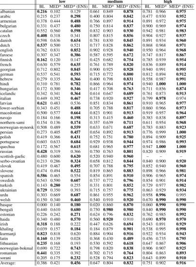
Table 2: Accuracies for task 1, for BL, MED* and MED* ensembles. Upper part: development languages; lower part: surprise languages.
8.2 MED Hyperparameters
We use the same hyperparameters for all MED models, i.e., all languages, tasks and amounts of resources. In particular, we keep them fixed to the following. Encoder and decoder RNNs each have 100 hidden units and the embeddings size is 300. For training we use ADADELTA (Zeiler,
Task 1 Task 2
Low 100 535
Medium 994 2285
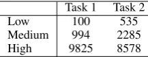
[image:7.595.125.234.62.104.2]High 9825 8578
Table 3: Average amount of training examples per task and resource quantity.
the best numbers obtained on the development set during training (“early stopping”). We compare the 1-best accuracy of all systems, i.e., the per-centage of predictions that match the true answer exactly.
8.3 Data
The official shared task data consists of sets for 52 different languages, 2 tasks and 3 different settings with varying amount of resources.3 An overview
of the (averaged) amount of samples per task and setting is given in Table3. Development and test sets are the same for all settings for each respective task and language. The gold labels for the test set are not published yet, so the experiments in this paper are performed on the development set.
8.4 Results
We compare our approaches to the official shared task baseline. Detailed results for task 1 and task 2 are shown in Table2and Table4, respectively.
Task 1. Table 2 shows the results obtained by
MED*, both for single models and ensembles. As can be seen, MED* already outperforms the base-line for the majority of languages in all settings; in average by 0.035, 0.157and0.151, respectively.
MED*’s performance is worse for the low data quantity than for the others. This is an expected result, as neural networks are known to require a huge amount of training instances.
Ensembling increases the final accuracy for all settings, by an average of 0.035 (low), 0.028
(medium) and0.014(high).
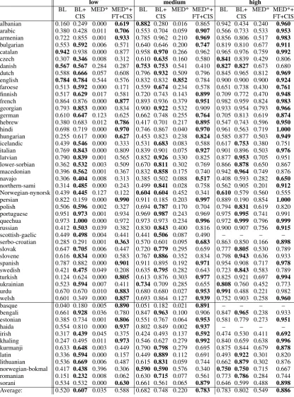
Task 2. As can be seen in Table4, combining BL
and CIS outperforms BL on its own for many lan-guages, especially in the low-resource setting. The highest improvements for the low-, medium- and high-resource setting are for Hungarian (0.362),
Latin (0.440) and Latin (0.429), respectively. For
some languages, e.g., Catalan, Danish or Urdu, choosing a good source form seems to not be im-portant. For a few languages, results even get
3A list of all languages can be found in Tables2and4.
worse. We will discuss some of those cases in§9. Overall, however, we obtain 0.087 (low), 0.066
(medium) and 0.019(high) improvement on
av-erage over all languages, which clearly shows the usefulness of CIS.
MED* on its own does not achieve competi-tive performance for task 2. We attribute this to the limited number of different lemmata given for training, resulting in an overfitting model, learn-ing, e.g., to produce certain character combina-tions for certain tags. However, MED*+FT+CIS outperforms both BL as well as BL+CIS for many languages in the medium- and high-resource set-tings and even in some low-resource scenarios. Comparing the obtained accuracies with Table1, it gets obvious that languages with a higher amount of given source forms per paradigm achieve bet-ter results afbet-ter fine-tuning, many times reaching a higher accuracy than BL, even in the low-resource setting. In contrast, fine-tuning works poorly for languages with ≤ 1.5 given source forms per
paradigm. In total, using MED*+FT+CIS, we ob-tain an average improvement of0.068(low),0.101
(medium) and0.103(high) over the baseline.
8.5 Official Shared Task Evaluation
Our submitted system obtained average accu-racies of 0.4659 (low), 0.8264 (medium) and 0.947(high) for task 1, and0.6776(low),0.8202
(medium) and 0.8852 (high) for task 2,
respec-tively. This corresponds to place 5 of 18, 3 of 19 and 7 of 15 for the high-, medium- and low-resource settings of task 1, respectively. Remark-ably, the difference to the best system for the two higher settings is less than0.01.
Among 3 submissions for task 2, our system comes first. It beats the baseline by 17.16(low), 15.54(medium) and10.84(high).
9 Remaining Challenges
Certain parts of our system do not perform as well for some languages as we would expect. In this section we will discuss those cases in more detail. CIS. For some languages, e.g., Danish or En-glish, CIS does not influence the performance. This might be due to those languages not having paradigm slots that are regularly closer to certain slots than others.
low medium high
BL BL+ MED* MED*+ BL BL+ MED* MED*+ BL BL+ MED* MED*+
CIS FT+CIS CIS FT+CIS CIS FT+CIS
albanian 0.160 0.249 0.000 0.619 0.882 0.280 0.016 0.865 0.942 0.434 0.240 0.960 arabic 0.380 0.428 0.011 0.706 0.553 0.704 0.059 0.907 0.566 0.733 0.533 0.953 armenian 0.722 0.855 0.001 0.933 0.785 0.962 0.210 0.969 0.856 0.806 0.517 0.983 bulgarian 0.553 0.592 0.006 0.571 0.640 0.646 0.200 0.747 0.819 0.810 0.677 0.911 catalan 0.942 0.938 0.000 0.877 0.958 0.970 0.266 0.962 0.965 0.976 0.759 0.992 czech 0.307 0.346 0.008 0.312 0.610 0.635 0.160 0.580 0.841 0.839 0.429 0.806 danish 0.567 0.567 0.284 0.287 0.753 0.753 0.541 0.410 0.827 0.827 0.673 0.680 dutch 0.588 0.666 0.057 0.608 0.796 0.932 0.509 0.796 0.845 0.965 0.812 0.969 english 0.784 0.784 0.544 0.576 0.832 0.832 0.852 0.784 0.900 0.900 0.900 0.924 faroese 0.513 0.592 0.000 0.171 0.559 0.674 0.234 0.578 0.651 0.738 0.430 0.761 finnish 0.517 0.629 0.017 0.581 0.720 0.743 0.143 0.899 0.709 0.772 0.470 0.948 french 0.864 0.876 0.000 0.877 0.893 0.936 0.379 0.951 0.982 0.959 0.824 0.983 georgian 0.793 0.853 0.000 0.834 0.900 0.922 0.532 0.909 0.933 0.954 0.793 0.966 german 0.610 0.647 0.123 0.625 0.662 0.748 0.255 0.764 0.705 0.813 0.619 0.874 hebrew 0.380 0.683 0.012 0.786 0.417 0.701 0.217 0.895 0.547 0.743 0.596 0.950 hindi 0.698 0.719 0.000 0.970 0.746 0.867 0.040 0.970 0.961 0.563 0.719 1.000 hungarian 0.255 0.617 0.000 0.627 0.453 0.823 0.238 0.824 0.585 0.877 0.503 0.949 icelandic 0.439 0.546 0.000 0.333 0.531 0.683 0.083 0.588 0.617 0.753 0.380 0.751 italian 0.769 0.843 0.000 0.809 0.839 0.901 0.075 0.927 0.901 0.896 0.503 0.976 latvian 0.790 0.839 0.001 0.565 0.852 0.926 0.330 0.825 0.877 0.953 0.705 0.951 lower-sorbian 0.362 0.532 0.003 0.509 0.670 0.811 0.302 0.769 0.866 0.878 0.650 0.867 macedonian 0.396 0.562 0.001 0.367 0.832 0.858 0.175 0.740 0.942 0.964 0.749 0.876 navajo 0.306 0.404 0.008 0.313 0.385 0.502 0.088 0.517 0.408 0.593 0.282 0.650 northern-sami 0.314 0.485 0.000 0.243 0.499 0.841 0.028 0.758 0.562 0.905 0.201 0.912 Norwegian-nynorsk 0.439 0.445 0.127 0.122 0.604 0.604 0.452 0.341 0.610 0.579 0.560 0.555 persian 0.822 0.159 0.000 0.990 0.911 0.185 0.203 0.997 0.889 0.190 0.854 1.000 polish 0.506 0.596 0.002 0.327 0.694 0.787 0.170 0.704 0.794 0.831 0.619 0.820 portuguese 0.951 0.973 0.001 0.934 0.969 0.987 0.243 0.969 0.975 0.995 0.741 0.991 quechua 0.973 1.000 0.000 0.972 0.973 0.973 0.234 0.996 0.972 0.999 0.796 0.999 russian 0.412 0.503 0.039 0.382 0.830 0.843 0.400 0.816 0.900 0.907 0.756 0.915 scottish-gaelic 0.449 0.498 0.004 0.441 0.441 0.506 0.087 0.490 – – – – serbo-croatian 0.285 0.291 0.001 0.363 0.570 0.601 0.095 0.683 0.863 0.850 0.166 0.898 slovak 0.647 0.705 0.006 0.447 0.720 0.779 0.295 0.659 0.777 0.805 0.530 0.789 slovene 0.616 0.834 0.000 0.583 0.767 0.886 0.352 0.834 0.798 0.943 0.636 0.933 spanish 0.787 0.882 0.000 0.901 0.911 0.895 0.192 0.971 0.954 0.908 0.717 0.978 swedish 0.421 0.475 0.049 0.208 0.635 0.795 0.282 0.643 0.723 0.843 0.583 0.789 turkish 0.124 0.624 0.000 0.805 0.613 0.876 0.303 0.977 0.825 0.921 0.697 0.994 ukrainian 0.523 0.594 0.007 0.411 0.734 0.709 0.285 0.655 0.808 0.760 0.452 0.773 urdu 0.670 0.670 0.010 0.883 0.680 0.680 0.027 0.953 0.991 0.488 0.221 0.982 welsh 0.601 0.349 0.000 0.857 0.693 0.864 0.127 0.939 0.752 0.903 0.258 0.960
basque 0.040 0.180 0.005 0.890 0.051 0.182 0.021 0.891 – – – –
bengali 0.661 0.928 0.036 0.780 0.847 0.963 0.100 0.906 0.847 0.965 0.238 0.933 estonian 0.385 0.734 0.001 0.806 0.551 0.767 0.064 0.953 0.581 0.779 0.273 0.951
haida 0.554 0.810 0.000 0.937 0.802 0.849 0.002 0.937 – – – –
[image:8.595.91.507.64.626.2]irish 0.317 0.439 0.045 0.375 0.424 0.493 0.137 0.592 0.474 0.530 0.411 0.692 khaling 0.247 0.495 0.011 0.973 0.546 0.627 0.279 0.992 0.840 0.659 0.638 0.996 kurmanji 0.633 0.648 0.003 0.449 0.790 0.798 0.279 0.695 0.875 0.844 0.679 0.878 latin 0.336 0.594 0.000 0.157 0.449 0.889 0.112 0.691 0.493 0.922 0.301 0.820 lithuanian 0.536 0.669 0.006 0.487 0.615 0.831 0.059 0.744 0.662 0.879 0.302 0.876 norwegian-bokmal 0.417 0.438 0.396 0.306 0.590 0.590 0.576 0.340 0.750 0.750 0.715 0.667 romanian 0.151 0.232 0.008 0.062 0.630 0.715 0.077 0.561 0.773 0.786 0.284 0.744 sorani 0.534 0.532 0.000 0.630 0.661 0.561 0.065 0.879 0.646 0.599 0.488 0.898 Average: 0.520 0.607 0.035 0.588 0.682 0.748 0.220 0.783 0.783 0.802 0.549 0.886 Table 4: Accuracies for task 2. All systems are described in the text. Upper part: development languages; lower part: surprise languages.
“riding a bike” and “hike”7→ “hiking” are not the same, even though they should be. Such cases po-tentially confuse the algorithm. A solution could be to detect training examples which consist of more than one token and split them up, in order to just consider the inflecting word.
Fine-tuning. For some settings and languages,
no forms of a paradigm are given. This results in the model being fine-tuned on autoencoding the lemma, and thus a strong bias to copy the input, which can hurt performance. A possible solution might be to apply a combination of fine-tuning and multi-domain training as proposed, e.g., by Chu et al. (2017) for neural machine translation. We leave respective experiments for future work.
10 Conclusion
We presented the LMU system for the CoNLL-SIGMORPHON 2017 shared task on universal morphological reinflection, which is based on an encoder-decoder network. We introduced two new methods for handling multi-source morphological reinflection: CIS, a source form selection algo-rithm based on edit trees and a fine-tuning ap-proach similar in spirit to domain adaptation. On average over all participating languages, our ap-proaches outperform the official shared task base-line for both tasks and all settings.
Acknowledgments
We would like to thank VolkswagenStiftung for supporting this research.
References
Roee Aharoni, Yoav Goldberg, and Yonatan Belinkov. 2016. Improving sequence to sequence learning for morphological inflection generation: The biu-mit systems for the sigmorphon 2016 shared task for morphological reinflection. InSIGMORPHON.
Dzmitry Bahdanau, Kyunghyun Cho, and Yoshua Ben-gio. 2015. Neural machine translation by jointly learning to align and translate. InICLR.
Kyunghyun Cho, Bart Van Merri¨enboer, Dzmitry Bah-danau, and Yoshua Bengio. 2014a. On the proper-ties of neural machine translation: Encoder-decoder approaches. arXiv preprint 1409.1259.
Kyunghyun Cho, Bart Van Merri¨enboer, C¸alar G¨ulc¸ehre, Dzmitry Bahdanau, Fethi Bougares, Hol-ger Schwenk, and Yoshua Bengio. 2014b. Learning phrase representations using RNN encoder–decoder for statistical machine translation. InEMNLP.
Grzegorz Chrupała. 2008. Towards a machine-learning architecture for lexical functional grammar parsing. Ph.D. thesis, Dublin City University.
Chenhui Chu, Raj Dabre, and Sadao Kurohashi. 2017. An empirical comparison of simple domain adapta-tion methods for neural machine translaadapta-tion. arXiv preprint 1701.03214.
Ryan Cotterell, Christo Kirov, John Sylak-Glassman, G´eraldine Walther, Ekaterina Vylomova, Patrick Xia, Manaal Faruqui, Sandra K¨ubler, David Yarowsky, Jason Eisner, and Mans Hulden. 2017a. The CoNLL-SIGMORPHON 2017 shared task: Universal morphological reinflection in 52 lan-guages. InCoNLL-SIGMORPHON.
Ryan Cotterell, Christo Kirov, John Sylak-Glassman, David Yarowsky, Jason Eisner, and Mans Hulden. 2016. The SIGMORPHON 2016 shared task— morphological reinflection. InSIGMORPHON.
Ryan Cotterell, John Sylak-Glassman, and Christo Kirov. 2017b. Neural graphical models over strings for principal parts morphological paradigm comple-tion. InEACL.
Manaal Faruqui, Yulia Tsvetkov, Graham Neubig, and Chris Dyer. 2016. Morphological inflection genera-tion using character sequence to sequence learning. InNAACL-HLT.
Dan Gusfield. 1997. Algorithms on strings, trees and sequences: computer science and computational bi-ology. Cambridge university press.
Katharina Kann and Hinrich Sch¨utze. 2016a. MED: The LMU system for the SIGMORPHON 2016 shared task on morphological reinflection. In SIG-MORPHON.
Katharina Kann and Hinrich Sch¨utze. 2016b. Single-model encoder-decoder with explicit morphological representation for reinflection. InACL.
Quoc V Le, Navdeep Jaitly, and Geoffrey E Hinton. 2015. A simple way to initialize recurrent networks of rectified linear units. CoRRabs/1504.00941. Minh-Thang Luong and Christopher D Manning. 2015.
Stanford neural machine translation systems for spo-ken language domains. InIWSLT.
Ilya Sutskever, Oriol Vinyals, and Quoc V Le. 2014. Sequence to sequence learning with neural net-works. InNIPS.
Matthew D Zeiler. 2012. ADADELTA: An adaptive learning rate method. CoRRabs/1212.5701.