Monte Carlo Simulation of
asymptotic approximation formula for the vanilla Euro-pean call option price. A class of multi-factor volatility models has been introduced which are driven by two dif-fusions, one fluctuating on a fast time scale and another one fluctuating on a slower time scale. It has been shown that it is possible to combine a singular perturbation ex-pansion with respect to the fast scale with a regular per-turbation expansion with respect to the slow scale. This again leads to a leading term which is the Black-Scholes price with a constant effective volatility.
Following the multi-factor stochastic volatility model in [7] and in [3], we consider the family of stochastic volatil-ity model, whereStis the underlying price,Ytevolves as
an Ornstein-Uhlenbeck (OU) process, andZtfollows
an-other diffusion process. Given the risk neutral probability measure P∗, the stochastic volatility model is described with the following equations:
dSt=rStdt+σtStdWt0 (1)
σt=f(Yt, Zt) (2)
dYt=
α(mf−Yt)−νf
√
2αΛf(Yt, Zt)
dt+ (3)
νf√2α
ρ1dWt0+
1−ρ21dWt1
.
dZt=
δ(ms−Zt)−νs
√
2δΛs(Yt, Zt)
dt+ (4)
νs
√
2δ
ρ2dWt0+ρ12dWt1+
1−ρ22−ρ212dWt2
.
Here (Wt0, Wt1, Wt2) are independent standard Brownian motions with instant correlation coefficientsρ1, ρ2, and ρ12 such that ρ21 < 1, and ρ22+ρ212 < 1, whereas St is the underlying stock price process with the risk free rate equal to r. The volatility process σt is driven by two
factors;YtandZt. As stated in [3] the risk neutral
prob-ability measureP∗ is determined by the market prices of volatility risk captured in Λf and Λs, which are assumed
to be bounded and independent of the stock priceS. The driving processes forYtandZtare mean reverting around
their long run mean mf and ms, respectively when Λf
and Λsare equal to zero. The mean reversion rate forYt
andZtareα >0 andδ >0 respectively, whereYtis fast mean reverting on a short time scale 1/αandZtis slowly varying on a long time scale 1/δ (i.e. α−1 <1 < δ−1). The time scales ofYtandZtare given as 1/αand 1/δwith the “vol-vol” parameter equal toνf√2αandνs√2δ, with long run distribution of OU process given as N(mf, νf2) andN(ms, νs2) as prototypes of more general ergodic
dif-fusions. Following Fouque and Han [3], in the numerical computations we use the the asymptotic theory in the mean reversion regime whereα→ ∞,δ→0.
LetH(ST) denote the payoff from an European call
op-tion, which is a function of the final stock priceST. Hence
under the risk neutral measureP∗ the no arbitrage price
is given by the conditional expectation of the discounted payoff given the current levels of (St, Yt, Zt):
P(t, x, y, z) =E∗
e−r(T−t)H(ST)|St=x, Yt=y, Zt=z
. (5) The crude Monte Carlo estimate of the option price is given by
P(t, x, y, z)≈ 1 N
N
k=1
e−r(T−t)H(S(k)
T ), (6)
whereST(k)is the price at maturity found by thekth sim-ulation using the Euler discretization of the process, and N is the total number of simulations.
2.1
Option Price Approximations
An approximation under the two-factor stochastic volatil-ity model is given by Fouque et al. [4] using the asymp-totic expansion theory. Asympasymp-totic expansion theory can be applied by introducing the parameter= 1/α. Hence, bothandδare small quantities such that 0< , δ <<1. We use a singular expansion aboutand a regular expan-sion aboutδ. By applying the Feynman-Kac formula to (5), the formula for P,δ can be obtained as given in [4]
with the price dependent onandδ. The pointwise price approximation is
P,δ(t, x, y, z)≈P(t, x, z), where
P =PBS(¯σ)+ (T−t)× (7)
V0 ∂ ∂σ +V1x
∂2
∂x∂σ +V2x 2 ∂2
∂x2 +V3x ∂ ∂x
x2 ∂2 ∂x2
PBS(¯σ),
with an accuracy of order (|log|+δ) for call options. The pricePBS(¯σ) is the homogenized price which solves
the Black-Scholes equation
LBS(¯σ)= 0 (8)
PBS(¯σ)(T, x) =H(x), (9)
where ¯σis called the effective volatility and is defined by
¯
σ2=< f2(., z)> . (10)
The brackets are used to denote the average with respect to the invariant distributionN(mf, ν2f) of the fast factor
(Yt). The parameters (V0, V1, V2, V3) are
V0=−νs
√
δ
√
2 Λsσ¯
, (11)
V1= ρ2νs
√
δ
√
2 fσ¯
, (12)
V2= νf
√
√
2 Λf ∂φ
∂y, (13)
V3=−ρ1νf
√
√
2 f ∂φ
where ¯σdenotes the derivative of ¯σ. The functionφ(y, z) is the solution of the Poisson equation
L0φ(y, z) =f2(y, z)−σ¯2(z).
Equation (7) gives us two approximations. The first is the actual solutionP and if we ignore all terms of order
√
, √δ or higher we get the first order approximation PBS(¯σ). It should also be noted that if a higher order approximation is desired it is possible to redo the asymp-totic expansion keeping more terms to get a higher order approximation, but the approximation will be much more complicated than the already complicatedP.
Table 1: Parameter values for our numerical experiments S0 Y0 Z0 K T r mf ms nf ns
55 -1 -1 50 1 1 -0.8 -0.8 0.5 0.8 ρ1 ρ2 ρ12 Λf Λs f(y, z) Δt N -0.2 -0.2 0 0 0 exp(y+z) 0.01 5000
3
Quasi-Monte Carlo (QMC) Method
The general problem for which QMC methods have been proposed as an alternative to the MC method is multidi-mensional numerical integration. One might consider the QMC method as the deterministic version of the Monte Carlo simulation. Convergence of the MC estimator is based on the central limit theorem, whereas in the QMC method a deterministic upper bound for the error is given by an upper bound.
The idea of QMC method is to use a more regularly dis-tributed point set, so that a better sampling of the func-tion can be achieved. An important difference with the MC method is that the point set PN is deterministic.
A detailed discussion of these methods can be found in Niederreiter [19]. The use of more “regular” or “uniform” points in the QMC method means these sequences satisfy certain uniformity conditions. A commonly used measure for uniformity of a QMC sequence is thestar discrepancy
D∗(PN) of a point setPN, which looks at the difference
between the volume of a rectangular box aligned with axes of [0,1)sand having a corner at the origin, and the
fraction of points fromPN contained in the box, and then the maximum difference over all such boxes. Typically, a point set PN is called a low discrepancy sequence if D∗(PN) = O(N−1logsN). For a function of bounded variation in the sense of Hardy and Krause, the integra-tion error|I−Iˆ|is inO(N−1logsN) when we use a low-discrepancy sequence in the integration (see Niederreiter [19] for details).
The convergence rate for QMC method by using low-discrepancy sequences suggests that if the dimension of the integration is high the advantages of QMC might be lost or more precisely QMC methods will require a very
large sample size when the dimensionsis high. However, we should note that our error analysis in QMC method is based on an upper bound for the error and for some problems with smooth integrands the observed conver-gence rate might be much faster than the converconver-gence rate of the upper bound. There are several studies in the literature showing this phenomenon some examples can be found in [1], [10], and [15].
3.1
Faure Sequence
In this subsection we describe the generation of a com-monly used quasi-Monte Carlo sequence, namely Faure sequence. Faure sequence has certain advantages for the valuation of high dimensional integrals, which leads to the efficient algorithms for the computation of complex financial derivatives. Applications of the Faure sequence in complex financial derivatives can be found in [12].
To compute the nth element of the Faure sequence, we start by representing any integern in terms of the base b,
n=
m
j=0
a1jbj. (15)
The first element of the Faure sequence is given by reflec-tion about the decimal point as before,
φ1b(n) =
m
j=0
a1jb−j−1. (16)
The remaining elements of the sequence can be found recursively. As also explained in Joy et al. [12], given akj−1(n) the next term can be written as
akj(n) =
m
j=1
Cjiaki−1(n) (modb), (17)
where Cji = j!(ii−!j)!. Hence, to generate the next di-mension in the sequence we multiply with the generator matrix, which is the upper triangular matrix with entries as the binomial coefficients,
⎛ ⎜ ⎜ ⎜ ⎜ ⎝
C00 C01 C02 C03 ... 0 C11 C12 C13
0 0 C22 C23 ... 0 0 0 C33
⎞ ⎟ ⎟ ⎟ ⎟ ⎠.
Hence, the rest of the points can be generated by,
φkb(n) =
m
j=0
akj(n)b−j−1, 2≤k≤d. (18)
We can represent the nth element of the ddimensional Faure sequence by,
0 0.2 0.4 0.6 0.8 1 0 0.1 0.2 0.3 0.4 0.5 0.6 0.7 0.8 0.9
1 Mersenne Twister
0 0.2 0.4 0.6 0.8 1 0 0.1 0.2 0.3 0.4 0.5 0.6 0.7 0.8 0.9
1 Faure Sequence
0 0.2 0.4 0.6 0.8 1 0 0.1 0.2 0.3 0.4 0.5 0.6 0.7 0.8 0.9
[image:4.595.75.252.96.166.2]1 Linear Scrambled Faure Sequence
Figure 1: Two dimensional projection of the gener-ated points from Mersenne Twister, Faure Sequence and Scrambled Faure Sequence (d1 = 1, d2 = 2, base= 2)
0 0.2 0.4 0.6 0.8 1 0 0.1 0.2 0.3 0.4 0.5 0.6 0.7 0.8 0.9
1 Mersenne Twister
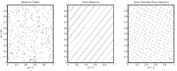
d1 = 5
d2 = 40
0 0.2 0.4 0.6 0.8 1 0 0.1 0.2 0.3 0.4 0.5 0.6 0.7 0.8 0.9
1 Faure Sequence
d1 = 5
0 0.2 0.4 0.6 0.8 1 0 0.1 0.2 0.3 0.4 0.5 0.6 0.7 0.8 0.9
1 Linear Scrambled Faure Sequence
d1 = 5
Figure 2: Two dimensional projection of the gener-ated points from Mersenne Twister, Faure Sequence and Scrambled Faure Sequence (d1 = 5, d2 = 40, base= 41)
Example 1 The following table displays the first ten
el-ements of the Faure sequence.
Construction of the Faure sequence
n a0(n) a1(n) a2(n) φ1n φ2n φ3n
1 1 0 0 1/3 1/3 1/3
2 2 0 0 2/3 2/3 2/3
3 0 1 0 1/9 4/9 7/9
4 1 1 0 4/9 7/9 1/9
5 2 1 0 7/9 1/9 4/9
6 0 2 0 2/9 8/9 5/9
7 1 2 0 5/9 2/9 8/9
8 2 2 0 8/9 5/9 2/9
9 0 0 1 1/27 16/27 13/27
10 1 0 1 10/27 25/27 22/27
3.2
Randomized Quasi-Monte Carlo
Quasi-Monte Carlo is based on the use of deterministic low discrepancy sequences with nice uniformity proper-ties. However, for two main reasons often we are inter-ested in using the randomized version of these sequences. First reason is the convenience of using confidence in-tervals while preserving much of the accuracy of pure quasi-Monte Carlo. Thus, randomized quasi-Monte Carlo method seeks to combine the best features of Monte Carlo and quasi-Monte Carlo methods. Secondly, there are set-tings in which randomizing a low discrepancy sequence actually improves accuracy. An important result show-ing that the root mean square error of integration usshow-ing a class of randomized nets is O(1/N1.5−), whereas the
error without randomization isO(1/N1−) for smooth in-tegrands. Even though Owen’s [18] result is restrictive in terms of pricing financial derivatives it is an important ex-ample to show that randomization can take advantage of the smoothness of the integrand which quasi-Monte Carlo alone cannot achieve. Discussion on improving accuracy through randomization of low discrepancy sequences can be found in Hickernell [11], Matousek [14], and L’Ecuyer and Lemieux [13].
It is often useful to randomize QMC point sets for the purpose of error analysis. Two desirable properties that a given randomization should have are: (i) each point in the randomized point set should have a uniform distribution on thes-dimensional hypercube; (ii) the uniformity of the original point set should be preserved.
Owen’s scrambling method is computationally demand-ing. Matou˘sek [14] introduced an alternative scrambling approach which is not only efficient but also satisfies some of the theoretical properties of Owen’s scrambled nets and sequences. In Owen’s scrambling is given in [18] and in
¨
Okten and Eastman [16]. Instead of Owen’s scrambling method we prefer to use the computationally less costly Matousek scrambling method (see Glasserman [9] for de-tails on scrambling quasi-Monte Carlo sequences).
As well known, quasi-Monte Carlo methods have better convergence rate, at least asymptotically, of O(logdN/N), whereas Monte Carlo methods have con-vergence rate ofO(N−1/2), whereN is the sample size
or the number of simulations. In many problems we do not have analytical formulas, this increased the popular-ity of quasi-Monte Carlo methods and special softwares has been designed for this purpose. Low discrepancy se-quences are deterministic, hence we get a single estimate of the result. This is a drawback for QMC method, since having many estimates of the unknown quantity we can construct confidence intervals. Furthermore, the deter-ministic error bound due to Koksma-Hlawka inequality is not computationally feasible for most of the problems. Therefore, computing the standard deviation and con-structing a confidence band for our estimates is quite desirable in a quasi-Monte Carlo simulation. To ad-dress this drawback of quasi-Monte Carlo methods, re-searchers introduced randomized versions of quasi-Monte Carlo methods, where we still have the good uniformity properties of low discrepancy sequences but also a statis-tical error analysis is available. A good discussion can be found in L’Ecuyer and Lemieux [13] and in ¨Okten and Eastman [16].
Estimate
I=
[0,1)d
[image:4.595.74.252.240.312.2]using sums of the form
Q(qu) = 1 N
N
n=1
f(qu(n)) (20)
wherequis a family ofd-dimensional low-discrepancy
se-quences indexed by the random parameteru.
Matou˘sek [14] proposes a linear digit scrambling method, by multiplying the generator matrix of a low discrepancy sequence by a random matrix for which entries consisting of 0,1,2, ..., b−1 and adding a random vectorU in mod b. This method is easier to implement compared to the full scrambling, and for thejth permutation it is applied to the digitaj by a simple choice ofπj given by
πj(aj) =hjaj+gj (mod b) (21)
where hj ∈ {0,1,2, ..., b−1} and gj ∈ {0,1,2, ..., b−1} are random integers.
Another choice is given by
πj(aj) = j
i=1
hijaj+gj (modb) (22)
which is used to generate the Generalized Faure sequence. Here, again the arithmetic is done in mode b, where gj and hij are selected at random and uniformly from
{0,1,2, ..., b−1}. In matrix notation, we can write the same expression as
π(a) =HTa+g
where HT is nonsingular lower-triangular matrix with
random entries. Matou˘sek [14] shows that scrambling methods both in Equations21and 22 preserves the net property.
In Figure 1 we plot the first two dimensions of a two dimensional uniform sequence. The first plot coming from the uniform random number generated by Mersenne Twister pseudo-random number generator. The second and third plots belong to the Faure sequence and its linear scrambled version. On Figure2we plot a two dimensional projection of a 40 dimensional sequence for the first 500 forty dimensional vectors. Figure2shows that when we plot dimension 5 versus dimension 40 coming from these 40 dimensional vector of points, Faure sequence starts to show linear patterns. These linear patterns are undesir-able in an integration problem since the “good quality” of the Faure sequence is lost as the dimension gets higher. On the same figure, the third plot shows that the lin-ear scrambled Faure sequence still preserves most of the uniformity of the Faure sequence at higher dimensions. Therefore, scrambling a low-discrepancy sequence such as the Faure sequence gives us the chance to deal with high dimensional problems without losing the nice fea-tures of the original low-discrepancy sequence.
4
Numerical Results
The multi-stochastic volatility model discussed is applied to the vanilla European option pricing problem with the given parameter values in Table1. This problem is used for both testing the effectiveness of importance sampling with tilting parameters derived from the Black-Scholes model and asymptotic approximation methods. Fur-thermore, randomized quasi-Monte Carlo sequences are tested in this high dimensional problem. As given in Table 1 Δt = 0.01 and T = 1, thus we have 100 time increments (T /Δt) in each simulated path of the process, requiring the use of 300 dimensional quasi-Monte Carlo sequence at each sample path. Thus, the dimension of the problem is very high for expecting good performance from the quasi-Monte Carlo simulation. For the crude Monte Carlo, results are obtained using the Mersenne twister pseudo-random number generator. For generating the normal deviates Box Muller transformation is used as discussed in [17].
[image:5.595.301.536.424.479.2]In our numerical experiments we used the digit scram-bling given Equation 21 and linear scrambling given in Equation22.
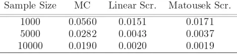
Table 2: European Call Option RMSE: MC versus RQMC
Sample Size MC Linear Scr. Matousek Scr.
1000 0.0560 0.0151 0.0171
5000 0.0282 0.0043 0.0037
10000 0.0190 0.0020 0.0019
The randomized quasi-Monte Carlo method is then ap-plied to our vanilla European call option pricing problem under the two factor stochastic volatility model. Room mean squared error (RMSE) results show that the best performer is Matousek scrambled Faure sequence at sam-ple sizes 5000 and 10000. At a samsam-ple size of 1000 lin-ear scrambled Faure sequence performed best. By us-ing the scrambled Faure sequence we observed factors of improvement around 6-10 compared to the crude Monte Carlo variance. Overall, both scrambling methods were superior to the crude Monte Carlo estimator with small differences between two scrambling methods.
5
Conclusion
sequence outperforms the crude Monte Carlo estimator by offering significant reductions in the variance.
References
[1] R. E. Caflish, W. Morokoff, and A. B. Owen, Valu-ation of mortgage-backed securities using Brownian bridges to reduce effective dimension, The Journal of Computational Finance, 1 (1) (1997), pp.27-46. 3
[2] Christoffersen, Peter, Heston, Steven L. and Jacobs, Kris, The Shape and Term Structure of the Index Option Smirk: Why Multifactor Stochastic Volatil-ity Models Work so Well (February 20, 2009). Avail-able at SSRN: http://ssrn.com/abstract=9610371
[3] J. P. Fouque and C. H. Han, Variance reduction for monte carlo methods to evaluate option prices under multi-factor stochastic volatility models, Quantita-tive Finance, 4 (2004), pp. 597606. 1,2, 2
[4] J. P. Fouque, G. Papanicolau, and K. R. Sircar, Derivatives in Financial Markets with Stochastic Volatility, Cambridge University Press, Cambridge UK, 2000. 1,2.1,5
[5] J. P. Fouque, G. Papanicolaou, R. Sircar, and K. Solna, Short time-scale in SP500 volatility, Jour-nal of ComputatioJour-nal Finance 6, pp. 1-23, 2003. (document),1
[6] J. P. Fouque, G. Papanicolaou, R. Sircar, and K. Solna, Singular perturbations in option pricing, SIAM J. Appl. Math., 63, pp 1648-1665, 2003. 1
[7] J. P. Fouque, G. Papanicolaou, K. R. Sircar, and K. Solna, Multiscale stochastic volatility asymptotics, SIAM Journal on Multiscale Modeling and Simula-tion, 2 (2004), pp. 2242. 1,2
[8] J. P. Fouque and T. A. Tullie, Variance reduction for monte carlo methods in a stochastic volatility envi-ronment, Quantitative Finance, 2 (2002), pp. 2430.
[9] P. Glasserman, Monte Carlo Methods in Financial Engineering, New York Springer, 2004. 3.2
[10] A. G¨onc¨u, Monte Carlo and quasi-Monte Carlo Methods in Financial Derivative Pricing, PhD. Dis-sertation, Florida State University, 2009. 3
[11] F. J. Hickernell (1996), The mean square discrep-ancy of randomized nets, ACM Transactions on Modeling and Computer Simulation, 6, 274-296. 3.2
[12] C. Joy, P. P. Boyle, and K. S. Tan (1996), Quasi-Monte Carlo Methods in Numerical Finance, Man-agement Science, 42, 926-938. 3.1,3.1
[13] P. L’Ecuyer, and C. Lemieux (2000), Variance re-duction via lattice rules, Management Science, 46, 1214-1235. 3.2
[14] J. Matousek (1998), On theL2-discrepancy for an-chored boxes, Journal of Complexity, 14, 527-556. 3.2,3.2,3.2
[15] G. ¨Okten, E. Salta, and A. G¨onc¨u, On pricing dis-crete barrier options using conditional expectation and importance sampling Monte Carlo, Mathemati-cal Modelling and Computation, 47, 484-494, 2008. 3
[16] G. ¨Okten and W. Eastman, Randomized quasi-Monte Carlo methods in pricing securities, Journal of Economic Dynamics and Control Volume 28, Issue 12, December 2004, Pages 2399-2426 3.2
[17] G. ¨Okten and A. G¨onc¨u, Generating low-discrepancy sequences from the normal distribution: Box Muller or inverse transform?, Mathematical and Computer Modelling, Volume 53, 2011, Pages 1268-1281 4
[18] A. B. Owen, Scrambled net variance for integrals of smooth functions, Annals of Statistics, 25, 1541-1562, 1997. 3.2