Abstract— In this paper a non-linear predictive controller with an empirical internal model based on Artificial Neural Networks (ANNs) is proposed. The ANN has high non-linear approximation capability and makes possible the use of plant information to generate future control actions. The results show the high potential of the proposed procedure when applied to the continuous extractive fermentation process of bioethanol production, an integrated reaction-separation process with highly complex non-linear dynamics.
Index Terms— Artificial neural networks, continuous
extractive fermentation process, non-linear predictive control.
I. INTRODUCTION
HE increasing demand for energy caused by the global economic growth generates a series of environmental problems and, in this context, there is a great interest in developing technologies for sustainable bioenergy production.
Among several options, the ethanol obtained by fermentation of sugarcane is an attractive biofuel to be used as a substitute for gasoline and can help to reduce gas emissions that produce the greenhouse effect [1]. This characteristic has increased the demand for bioethanol, which makes the development of more efficient production technologies desirable. One alternative is to apply process intensification techniques in continuous production processes. Integrated processes of reaction-separation provide alternative solutions [2], such as the production of ethanol by fermentation with a continuous withdrawal of the ethanol produced using a flash separation unit. This action regulates the concentration of ethanol in the fermentor to ranges where the inhibitory effect of the product on the yeast activity decreases, improving the process productivity [2] [3] [4]. However, these bioprocesses are highly nonlinear, its mathematical modeling is complex and there are additional difficulties to calculate the vapor-liquid equilibrium due to the composition of the fermented liquid [5]. These characteristics also make the use of classical control techniques to control the process difficult [6]. In this
Manuscript received July 16, 2011; revised August 03, 2011. This work was supported in part by the CAPES and FAPESP.
E.G. Boza-Condorena is the corresponding author.Phone: 19-8119-1822;
e-mail: ebozac2003@ yahoo.es. He is with the School of Chemical Engineering, State University of Campinas, 13083-970, Campinas, SP, Brazil
D.I.P. Atala is with Centro de Tecnologia Canavieira, 13400-970-Piracicaba,SP, Brasil
A.C. da Costa is with the School of Chemical Engineering, State University of Campinas, 13083-970, Campinas, SP, Brazil. (e-mail: [email protected]).
paper neural network model predictive controllers, NNMPC, are designed to control the continuous production process of bioethanol by fermentation and separation via flash evaporation. The controller is based on the dynamic matrix control (DMC) algorithm, which is representative of the MPC technology [7] [8].
II. PROCESS DESCRIPCION
A. Experimental Stage
The research experimental stage was conducted at the Bioprocess Engineering Laboratory of the State University of Campinas, Brazil.
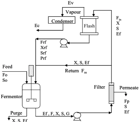
[image:1.595.311.548.419.626.2]The extractive fermentation process is integrated by: one reaction unit (fermentor), one cell recycle system (cross-flow microfiltration), one vacuum separation system (flash tank for ethanol-fermented broth separation and vacuum pump), two helical pumps, three peristaltic pumps, and one condensing unit. The total working volume is approximately 5 L. Fig. 1 shows a diagram of the extractive fermentation process with vacuum flashing [4].
Fig. 1. Diagram of the extractive fermentation process with vacuum flashing
A 3 liters "Bioflo III System" (New Brunswick Scientific Co., Inc., NJ, USA) bioreactor with PID (Proportional, Integral and Differential) control of temperature and agitation was used as the reaction unit. A cross-flow microfiltration unit (Ceraflow model, Millipore Co.) with a filter element made of high purity alumina, 0.22 mm pore and 0.0372 m2 filtration area was used in the cell
recycle system. The flash tank was a 2.5 liters (working volume) adapted Chemap reactor. The device to measure the input flow was an electromagnetic flowmeter (IFS 400 KC
Non-linear Predictive Control of a Fermentor in
a Continuous Reaction-separation Process
Edwin G. Boza-Condorena, Daniel Ibraim Pires Atala , and Aline Carvalho da Costa
T
Flash
Permeate Filter
Feed
Fermentor
Return Fre
Vapour
Ef , F, X, S, G Fo
So
Fp S Ef
X, S, Ef
X, S, Ef
Fin X S Ef Ec
Frf Xrf Srf Prf
Purge
Condenser Ev
Flash
Permeate Filter
Feed
Fermentor
Return Fre
Vapour
Ef , F, X, S, G Fo
So
Fp S Ef
X, S, Ef
X, S, Ef
Fin X S Ef Ec
Frf Xrf Srf Prf
Purge
model, signal converter IFC 090 model; Conaut, Brazil) with an operating range from 0 to 1200 L/h. Temperature in the fermentor and flash tank was measured using K type thermocouples (N. Brunswick Scientific Co.). A Cold trap, -25 ºC working temperature (MA-055 model, Marconi laboratory equipment, Brazil), was used in the condensing system.
The yeast used was Saccharomyces cerevisiae obtained from an industrial fermentation plant. The medium used in the fermentation was sugarcane molasses containing about 77% of purity in sugar, diluted in water with to a concentration of 180 g / L of reducing sugars.
A stage of batch fermentation was initiated shortly after the addition of the inoculum. The objectives in this stage were to promote the total consumption of substrate and to reach a high biomass concentration before the second stage begins. The end of the batch fermentation stage was observed by the stabilization of turbidity and condensate volume readings. The continuous extractive fermentation was initiated by turning on the permeate pump of the filtration system. The removal of fluid with the permeate and purge pumps decreased the fermentation broth level into the fermentor activating the feeding pump (connected to an on-off level controller) that supplied fresh medium, by this action the level was kept constant throughout the fermentation.
The temperature in the fermentor was maintained constant at 33.25 ± 0.25 ºC, the feed of substrate concentration was constant at 180 g/L throughout the fermentation process, while the dilution rate of the fermentor was maintained constant in the levels of 0.03 h -1(33.33 h residence time), 0.10 h-1(10 h residence time),
0.15 h-1(6.67 h residence time), 0.20 h-1(5 h residence time)
and 0.35 h-1(2.85 h residence time). Working with this last
dilution rate it was possible to obtain a productivity of 25 g/L h, which is three times higher than the value obtained in the traditional fermentation process. The flash tank was operated with a feed flow rate of 200 L/h, vacuum pressure at 150 ± 40 mmHg, temperature at 33.8±0.4 ºC. The liquid remaining in the flash tank containing the fermentation broth with lower concentration of ethanol returned to the fermentor using a helical pump.
B. Variables selection
In this work two control alternatives using the model-based approach to control system design [9] were compared. The control objective is to regulate the ethanol concentration in the fermentor (Ef). In order to design the controller an empirical dynamic model of the process based on ANN was previously developed This approach was used instead of developing a phenomenological model of the process, as the modeling of the flash tank has been shown to be complex [5] and lead to inaccurate results.
After a preliminary study of the process, the following variables were considered as input variables to develop the model : 1) Permeate flow rate (FP) ; 2) Fermentor purge
flow rate (FPU); 3) Feed flow rate to the fermentor (F0); 4)
Fermentor biomass concentration (X) ; 5) Fermentor substrate concentration (S); 6) Residence time (tr) or Fermentor dilution (D=1/tr); 7) Fermentor Glycerol
concentration (G); 8) Cell viability (Cv); 9) Fermentor outlet flow rate (F); 10) Fermentor temperature (Tferm); 11)
Flash tank inlet flow rate (Fin); 12) Flash tank temperature
(Tflash); and 13) Flash tank pressure (Pflash).
III. MODELING AND CONTROL
A. Artificial Neural Network Modeling
A two layer feedforward network was employed to model the process with a tan–sigmoid transfer function on the hidden layer and a linear transfer function on the output layer, because according to Cybenko’s theorem, with this structure, the ANN models are able to approximate continuous functions at any desired level [10] [11]. The Levenberg-Marquardt method for backpropagation training was used to train the ANN.
In the ANN structure selected theinputs,
x
i, theweights that connect inputs to neurons in the hidden layer, Wji, theweights that connect neurons in the hidden layer to neurons in the output layers, Wkj, the bias, b, the activation
functions,
f
, and the value of the output variableE
kO are related by the following equation:
2
1 1
1 1
2
k N
j
M
i
j i ji kj
O
k f W f W x b b
E (1)
Where: j = 1,…, N (hidden layer neurons) ; i = 1,…, M (inputs); k = 1,…, K (output layer neurons). The weight Wji,
connects the ith input (xi), and the jth neurons on the hidden
layer (layer 1). The weight Wkj, connects the jth neuron of
the hidden layer, and the kth neurons of the output layer (layer 2). Superscript 1 indicates layer 1. Superscript 2 indicates layer 2, Superscript o indicates output layer. The ethanol concentration estimated in the kth neuron of the output layer is represented by
E
kO.The number of neurons in the hidden layers was determined by selecting the lowest mean square error (mse) when using the cross-validation technique, which is used to avoid model overfitting and to evaluate the performance of neural network by its ability to predict the elements of a validation dataset which was not used when training the neural network. In the present work a representative data base containing 800 input/output patterns corresponding to 400 h of continuous flash fermentation at different dilution rates (0.1, 0.15, 0.20 and 0.35 h-1
) was used; 600
input/output patterns (75%) were used for ANN training and the remaining 200 input/output patterns (25%) was used to validate the trained ANN.
B. Neural Network Model Predictive Control (NNMPC) algorithm
In the NNMPC algorithm proposed in this work the
convolution model used in the linear DMC algorithm is substituted by a non-linear internal model based on ANN, which is trained using data (input/output patterns) generated by the ANN model of the process. The predictive controller estimates a control action sequence (future inputs) that leads the controlled variables (outputs) to follow an optimal path to achieve a reference trajectory. This optimal path is determined by optimizing the following quadratic objective function [14] [15].
21 1 2 2 1
NCi k i NP
i k
c i
k ysp u
y
J
(2)Where:
ysp= set point,
= weighting factor (suppression factor), which prevent large swings in the manipulated inputs,
u
= value of the future change in the manipulated variable that minimize the performance indexJ
on the control horizon NC.c
y
= prediction made by the neural network model on a prediction horizon NP, corrected according to (7).Certain restrictions on the changes of the manipulated variable are also considered, so the optimal control action sequence is obtained by solving a constrained quadratic programming (QP) problem at each sampling time.
The optimization problem is written as a quadratic program:
U
f
U
H
U
U
T
T
(
)
(
)
2
1
)
(
min
(3)Subject to:
T(
U
)
(4)max
min
U
U
U
(5)Where the matrices
H
and
, are related to tuning parameters [16].
Ti k
u
U
1
(6)(k = sampling instant; i = 1,…, NC)
The vectorsη and
U
are linear functions of the output prediction vector, y, as well as of the tuning parameters.Although the future control actions are calculated over a control horizon NC
(
NC
NP
)
, only the first control action is utilized. The optimization algorithm was implemented in Matlab using the quadprog routine of the optimization toolbox.The algorithm uses a corrected value for the prediction
c
y
in (2), incorporating a feedback strategy. At instant k, the predicted value of the output is compared to the measured value; the difference is used to correct the predicted value ŷ in the NP moments ahead. For example, for the moment k + i:)
ˆ
(
ˆ
k i k kc i
k
y
y
y
y
(7)IV. RESULTS AND DISCUSSION
A. Process Modeling
Neural networks of configurations 13: N: 2, where N is the number of neurons in the hidden layer (N Є [6,10]), were tested in order to select the best ANN based model of the process. The lowest mse and R2 values obtained when
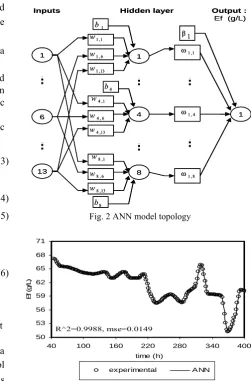
pairing the experimental validation set with the ANN predicted values were used as indicators of the best model. A neural network with topology 13:8:1, with 8 neurons in the hidden layer led to the lowest mse and R2 values, so it
[image:3.595.286.538.246.628.2]was selected as a model of the process. Fig. 2 shows the selected ANN model topology. Fig. 3 shows the high prediction performance of the model to values of the validation data set.
Fig. 2 ANN model topology
R^2=0.9988, mse=0.0149 50 53 56 59 62 65 68 71
40 100 160 220 280 340 400
time (h) E f ( g /L ) experimental ANN
Fig. 3. Output of ANN process model and experimental values of the validation data set.
B. Dynamic Behavior Study
A procedure to determine the effect of input variables, on the output variables is by making changes or disturbances in the values of the inputs one by one and observing the changes in the outputs. In this work random disturbances were made on the selected inputs one by one by simulating the dynamic behavior of the process.
As inputs were utilized: a) purge flow rate, b) permeate flow rate, c) feed flow rate to the fermentor, and d) the
6 1 1 4 8 6 , 4 w 1 , 4 w 1 , 8 w 6 , 8 w 13 , 8 w 1 , 1 w 6 , 1 w 1 b 4 b 8 b 4 , 1 ω 1 , 1 ω 1 β
Inputs Hidden layer Output :
Ef (g/L) 1 13 13 , 4 w 8 , 1 ω 13 , 1 w 6 1 1 4 8 6 , 4 w 1 , 4 w 1 , 8 w 6 , 8 w 13 , 8 w 1 , 1 w 6 , 1 w 1 b 4 b 8 b 4 , 1 ω 1 , 1 ω 1 β
Inputs Hidden layer Output :
fermentor dilution; and as output it was used the fermentor ethanol concentration, Ef.
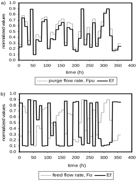
The highest associations between variables were obtained in two cases: 1) between the purge flow rate, Fpu, and the ethanol concentration in the fermentor, Ef, with a correlation coefficient, R = 0.99 and a range of variation of the output as a result of the variations in the input, r = 13.48 g/L (r=max(output)-min(output)) and 2) between the feed flow rate to the fermentor, Fo, and the ethanol concentration in the fermentor, Ef, with a correlation coefficient, R = -0.91 and a range of variation of the output as a result of the variations in the input, r = 28.22 g/L. Therefore Fpu and Fo could be appropriate variables to be considered as manipulated variables in order to control Ef.
Fig. 4 show graphically the behavior of the inputs: purge flow rate, Fpu, and feed flow rate to the fermentor, Fo; and the output ethanol concentration in the fermentor, Ef, with normalized values in the range [0.1, 0.9].
a)
0.0 0.1 0.2 0.3 0.4 0.5 0.6 0.7 0.8 0.9 1.0
0 50 100 150 200 250 300 350 400
tim e (h)
no
rm
a
li
z
ed
v
a
lue
s
purge flow rate, Fpu Ef
b)
0.0 0.1 0.2 0.3 0.4 0.5 0.6 0.7 0.8 0.9 1.0
0 50 100 150 200 250 300 350 400
tim e (h)
nor
m
al
iz
ed v
al
ues
[image:4.595.51.285.288.595.2]feed flow rate, Fo Ef
Fig. 4. Normalized values of inputs and outputs: a) Purge flow rate, Fpu, and ethanol concentration, Ef.
b) Feed flow rate to the fermentor, Fo, and Fermentor ethanol concentration, Ef.
From the results two NNMPC controller structures were proposed: control structure 1 with the purge flow rate, Fpu, as manipulated variable, and control structure 2 with the feed flow rate to the fermentor, Fo, as manipulated variable. The controlled variable is the ethanol concentration in the fermentor, Ef.
C. Internal Model Training
The DMC algorithm uses an internal model (convolution model) to generate predictions of future control actions. In this work the internal model is a neural network with two
inputs: the controlled and manipulated variables at the present sampling instant, t, and one output: the controlled variable one step ahead, (t +1). The training data (input/output patterns) were obtained by making 24 successive random disturbances on the inputs of the process model and determine the respective output. The interval between disturbances was chosen to ensure that the system reaches new steady states, as suggested by Santos and Biegler [17]. The internal model based on ANN has a 2:4:1 topology with 4 neurons in the hidden layer. The model performance in describing the training data was determined using the following equation, which was suggested by Milton and Arnold [18]:
%
100
)
1
(
S
SEE
corr
(8)WhereSEE k k
k N
( ( )ye y( )) 12,
S k
k N
( ( )ye ye) 12
,
ye(k) is an experimental output, y(k) is the corresponding
output of the neural model, ye is the average of experimental outputs and N is the number of experimental data. The two internal models describe the training data with correlations (corr) of: 99.05%, and 99.12%; respectively.
Another test suggested by various authors [15] [17] [19] and that was done with satisfactory results was to determine each model's ability to predict steady states of the process.
The practical experience from the present work has shown that additionally two more characteristics are important when testing the performance of the ANN internal model: 1) an accurate open loop response, and 2) a wide operation range.
D. Controller Performance
The predictive controllers with nonlinear internal model based on neural networks were subjected to various tests, considering a sampling time of 10 minutes. The parameter values were determined by trial and error; and comparing the controller performance in different cases:
1) Control structure 1 (manipulated variable: purge flow rate): prediction horizon, NP =10, control horizon, NC=3, λ = 0.22.
2) Control structure 2 (manipulated variable: feed flow rate to the fermentor): prediction horizon, NP =10, control horizon, NC=1, λ = 0.05.
Regulator Performance
54 56 58 60 62 64 66
0 25 50 75 100 125 150
tim e (m in)
E
f (
g
/L
)
-5%Fo NC=3 +5%Fo NC=3
-5%Fo NC=1 +5%Fo NC=1
[image:5.595.54.283.273.438.2]s etpoint
Fig. 5. Control structure 1: Response of the controlled variable, Ef, with time to perturbations of 5 % in the feed flow rate to the fermentor, Fo. Manipulated variable: purge flow rate, Fpu.
63.6 63.8 64 64.2 64.4 64.6 64.8 65 65.2
0 25 50 75 100 125 150
tim e (m in)
E
f (
g
/L
)
+20%Fpu NC=2 -20%Fpu NC=2
+20%Fpu NC=1 -20%Fpu NC=1
setpoint
Fig. 6. Control structure 2: Response of the controlled variable, Ef, with time to perturbations of 20 % in the purge flow rate, Fpu. Manipulated variable: feed flow rate to the fermentor, Fo.
Figs. 5 and 6 show that both NNMPC structures reject the disturbance and bring the system back to the steady state; therefore they have good regulatory performance. Three criteria were useful to describe the regulatory performance of the controllers: 1) the maximum deviation of the response from the reference trajectory, 2) the settling time, and 3) the IAE criterion (integral of the absolute value of the error), which provides controller settings that are between the most conservative settings, given by the ITAE criterion (integral of the time-weighted absolute error) and the most aggressive settings, given by the ISE criterion (integral of the squared error) [9]. Fig. 5 show that NC=3, is the best selection for control structure 1, and Fig. 6 show that NC=1, is the best selection for control structure 2. The deviation (d) from the reference trajectory is higher for control structure 1 (d=5.66) than for control structure 2 (d = 0.90). The settling time, defined as the time to reach 5% of the maximum deviation, is 50 min for control structure 1 (NC=3) and 30 min for control structure 2 (NC=1). Control structure 1 leads to a higher IAE value (IAE=104.98) than control structure 2 (IAE=13.55).
From the tests that were realized we can state that a carefully determination of the: “dynamic matrix” elements, suppression factor λ, control horizon NC, and prediction
horizon NP, is important to increase the performance of the NNMPC controllers. Although control structure 2 appears to have the best regulatory performance, it is necessary to do more tests using different disturbances of similar magnitude in order to have a better conclusion. In the present case there are strong interactions between input variables, e.g. feed flow rate to the fermentor, Fo, and permeate flow rate, Fp; Fermentor dilution, D, and Fo; that give difficulty in stating a definitive conclusion.
Servo Performance
In this case successive changes were made in the value of the setpoint.
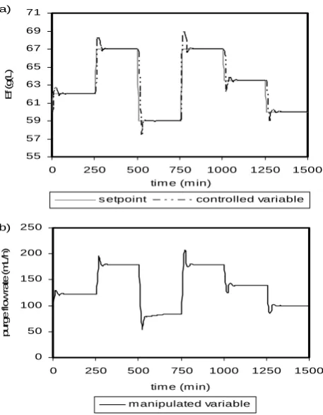
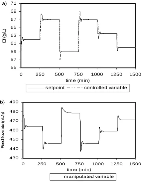
Figs. 7 and 8 show the behavior of the predictive controllers with neural internal model to various changes in the reference trajectory (setpoint). It is noted that both control structures performed well, bringing the system back to the steady state after each change in the setpoint (represented in this case by ethanol concentration in the fermentor, Ef).
a)
55 57 59 61 63 65 67 69 71
0 250 500 750 1000 1250 1500
tim e (m in)
Ef
(
g
(L
)
s etpoint controlled variable
b)
0 50 100 150 200 250
0 250 500 750 1000 1250 1500
tim e (m in)
pur
ge f
low
r
at
e (
m
L/
h)
[image:5.595.311.540.312.606.2]m anipulated variable
Fig. 7. Servo performance of the control structure 1: a) Controlled variable and setpoint changes
a)
55 57 59 61 63 65 67 69 71
0 250 500 750 1000 1250 1500
tim e (m in)
Ef
(
g
/L
)
s etpoint controlled variable
b)
430 440 450 460 470 480 490
0 250 500 750 1000 1250 1500
tim e (m in)
F
ee
d f
low
r
at
e (
m
L/
h)
[image:6.595.52.284.54.351.2]m anipulated variable
Fig. 8. Servo behavior of control structure 2: a) Controlled variable and changes in the setpoint. b) Manipulated variable (control actions).
V.
C
ONCLUSIONIn this paper a non-linear neural networks model predictive controller (NNMPC) was designed using the DMC algorithm. It was shown that the non-linear models based on ANN can accurately identify the experimental behavior of the studied process and have a good performance as the internal model in predictive controller.
The use of an ANN model to simulate the dynamic behavior of the process allowed the design of the proposed control system even when an accurate phenomenological model was not available. The predictive performances of the controllers were tested with load disturbances and setpoint disturbances with good results, which demonstrate the high potential of the procedures that have been used in this study for control system design in integrated reaction-separation processes.
R
EFERENCES[1] E. Smeets, M. Junginger, A. Faaij, A. Walter, and P. Dolzan. (2006, August). Sustainability of Brazilian Bio-ethanol. Utrecht University. Available: http://igitur-archive.library.uu.nl/chem/2007-0628-202408/NWS-E-2006-110.pdf
[2] C.A. Cardona and O.J. Sánchez, “Fuel ethanol production: Process design trends and integration opportunities,” Bioresour. Technol., vol. 98, no. 12, pp. 2415-2457, Mar. 2007.
[3] A. C. Costa, D. I. P. Atala, F. Maugeri, R. Maciel Filho, “Factorial design and simulation for the optimization and determination of control structures for an extractive alcoholic fermentation,” Process. Biochem., vol. 37, no. 2, pp.125-137, Mar. 2001.
[4] D.I.P. Atala, “Assembly, instrumentation, control and experimental development of an extractive fermentative process of ethanol production,” PhD dissertation, UNICAMP, SP, Brazil. 2004.
[5] V.H. Álvarez, E. Ccopa Rivera, A. C. Costa, R. Maciel Filho, M.R. Wolf Maciel, M. Aznar, “Bioethanol Production Optimization: A
Thermodynamic Analysis,” Appl. Biochem. Biotechnol., vol. 148, no.1-3, pp.141-149, Jan. 2008.
[6] A. Ashoori, B. Moshiri, A. Khaki-Sedigh, M. Reza, “Optimal control of a nonlinear fed-batch fermentation process using model predictive approach,” J. Proc. Cont., vol. 19, pp. 1162-1173, Mar. 2009. [7] D. Dougherty, D. A. Cooper, “A practical multiple model adaptive
strategy for single-loop MPC,” Control Eng. Practice, vol. 11, pp. 141–159, 2003.
[8] S. J. Qin and T.A. Badgwell, “A survey of industrial model predictive control technology,” Control Eng. Practice, vol. 11, no. 7, pp. 733-764, 2003.
[9] D.E. Seborg, T.F. Edgar and D.A. Mellichamp, Process Dynamics and Control, Second Edition, Hoboken, NJ: John Wiley & Sons, Inc., 2003.
[10] C.L. Nascimento and T. Yoneyama, Artificial Intelligence in Control and Automation, Sao Paulo, Brazil: Blucher- FAPESP. 2008. [11] E.C. Rivera, D. I. P. Atala, F. Maugeri, A. C. Costa, R. Maciel Filho,
“Development of real-time state estimators for reaction-separation processes: A continuous flash fermentation as a study case,” Chem. Eng. Proc.: Process intensification, vol. 49, pp. 402-409, Mar. 2010. [12] R. Scattolini. “Architectures for distributed and hierarchical Model
Predictive Control – A review,” J. Proc. Cont., vol. 19, pp. 723–731, Feb. 2009.
[13] Y. Zheng, S. Li, X. Wang. “Distributed model predictive control for plant-wide hot-rolled strip laminar cooling process,” J. Proc. Cont., vol. 19, pp. 1427-1437, Apr. 2009.
[14] W. Luyben. Process modeling, simulation and control for chemical engineers, Second Edition, New York, NY: McGraw-Hill, 1990. [15] A.C. Costa, R. Maciel Filho. “Non linear Predictive Control of a
Three-Phase Catalytic Reactor ,” Can. J. Chem. Eng., vol. 81, pp. 1109-1118, Oct. 2003.
[16] B.A. Ogunnaike and W.H. Ray. Process dynamics, modeling, and control, New York, NY: Oxford University Press, 1994.
[17] L.O. Santos, L.T. Biegler. “A tool to analyze robust stability for model predictive controllers,” J. Proc. Cont., vol. 9, pp. 233-246, 1999.
[18] J.S. Milton, J.C. Arnold. Introduction to Probability and Statistics, New York, NY: McGraw Hill, 1990.
[19] A.C. Costa, L.A.C. Meleiro, R. Maciel Filho. “Non-linear predictive control of an extractive alcoholic fermentation process,” Process Biochem., vol. 38, no. 5, pp. 743-750, Dec. 2002.