Measuring the compositionality of collocations via word co occurrence vectors: Shared task system description

Proceedings of the Workshop on Distributional Semantics and Compositionality (DiSCo’2011), pages 48–53,

Measuring the compositionality of collocations via

word co-occurrence vectors: Shared task system description

Alfredo Maldonado-Guerra and Martin Emms

School of Computer Science and Statistics Trinity College Dublin

Ireland

{maldonaa, mtemms}@scss.tcd.ie

Abstract

A description of a system for measuring the compositionality of collocations within the framework of the shared task of the Distribu-tional Semantics and ComposiDistribu-tionality work-shop (DISCo 2011) is presented. The system exploits the intuition that a highly composi-tional collocation would tend to have a consid-erable semantic overlap with its constituents (headword and modifier) whereas a colloca-tion with low composicolloca-tionality would share little semantic content with its constituents. This intuition is operationalised via three con-figurations that exploit cosine similarity mea-sures to detect the semantic overlap between the collocation and its constituents. The sys-tem performs competitively in the task.

1 Introduction

Collocations or multiword expressions vary in the degree to which a native speaker is able to under-stand them based on the interaction of their con-stituents’ individual meanings. The concept of com-positionality of a collocation captures this notion. The shared task of the DISCo 2011 workshop (Bie-mann and Giesbrecht, 2011) consists in comparing systems’ compositionality scores against composi-tionality scores based on human judgements. Sys-tems were evaluated on the match of the compo-sitional scores generated by the system and those based on human judgements – specifically taking the mean of the absolute difference of these scores. Ad-ditionally the organisers also classified the human-derived scores into three coarse categories of com-positionality: non-compositional (low), somewhat

compositional (medium) and compositional (high). Systems were required to produce an additional compositionality labelling into these three coarse categories and were evaluated on the precision of this labelling.

The methods used by our system for measuring compositionality take inspiration from the work of McCarthy et al. (2003), who measured the simi-larity between a phrasal verb (a main verb and a preposition likeblow up) and its main verb (blow) by comparing the words that are closely semanti-cally related to each, and use this similarity as an indicator of compositionality. Our method for mea-suring compositionality is considerably different as it instead directly compares the semantic similar-ity between the headword and the collocation and between the modifier and the collocation by com-puting a cosine similarity score between word co-occurrence vectors that represent the headword, the modifier and the collocation (see 3.2). Our system can be regarded as fully unsupervised as it does not employ any parsers in its processing or any external data other than the corpus and the collocation lists provided by the organisers.

The rest of the paper is organised as follows: Sec-tion 2 describes the corpora and the collocaSec-tion list provided by the task organisers. Section 3 intro-duces some definitions and describes the three con-figurations in detail. Section 4 presents the results and concludes.

2 Data

Shared task participants were provided with a list of collocations of three grammatical forms:

noun collocations (A-N), subject-verb collocations (S-V) and verb-object collocations (V-O). Our sys-tem assumes that each collocation consists of a headword and a modifier and it interprets these con-stituents in each grammatical form as follows:A-N: adjective - modifier, noun - headword;S-V: subject - modifier, verb - headword;V-O: verb - headword, object - modifier.

As a corpus, our system uses a random sample of 500,000 documents from the plain-text, non-parsed version of the English ukWaC corpus (Baroni et al., 2009).

3 System description

Our system can be employed in three different con-figurations. All three rely in representing words and collocations as word co-occurrence vectors and measure semantic similarity using the cosine mea-sure.

3.1 Preliminary definitions

These definitions are largely based on the con-struction of first-order context vectors, word co-occurrence vectors and second-order context vectors via global selection as described in Schütze (1998) and in Purandare and Pedersen (2004) by consider-ing context windows of 20 words centred at a target word.

Thefirst-order context vectoris a vector repre-senting atokenof a word, or equivalently aposition pin a document. Dimensions of the vector are word types w, and the value on dimension w is a count of the frequency with which w occurs in a specified window around p in a given document doc.

C1(p)(w) =

_∑

p06=p p−10≤p0 p0≤p+10

(1 ifw=doc(p0),else 0) (1)

In this work the dimensions are the 2,000 non-function words that are most frequent in the corpus1_. The word co-occurrence vector (or simply word vector) is a vector recording the co-occurrence be-haviour of a particular wordtype win a corpus. As

1_{We employ a modified version of the stop word}

list supplied with Ted Pedersen’s Text-NSP package (http://www.d.umn.edu/~tpederse/nsp.html)

such it can be defined by summation over first-order context vectors:

W(w) =

_∑

p

(1 ifw=doc(p),else 0)·C1(p) (2)

And thesecond-order context vectoris a further vector representing an instance of a word. For a par-ticular locationp, it is defined to besum of the word vectors of words in a given window around p

C2(p) =

_∑

p06=p p−10≤p0 p0≤p+10

W(doc(p)) (3)

Although the above are defined for types and to-kens ofwords, they can be generalised tomultiword

expressions in various ways. In this work, for any multiword expressiontype x y, its tokensare taken to be occurrences of the sequencexγy, whereγ can be any sequence of intervening words of length l, 0≤l≤3. By taking the position ofxas the position of the multiword token, and taking the first position after the token as position p+1, the definitions of

C1,WandC2can be carried over to multiword ex-pressions.

All the configurations described below use the co-sine measure between vectors, defined in the stan-dard way

cos(v,w) = ∑

N i=1viwi

q

∑Ni=1v2i∑ N i=1w2i

(4)

3.2 System configurations

For each collocation in the test set, thefirst configu-rationof our system starts off by building word vec-tors for the collocation, its headword and its modi-fier.

The first configuration of the system outputs the average of two cosine similarity measures as the compositionality score for the collocation:

c₁=1 2

cos(W(x y),W(x)) +cos(W(x y),W(y))

(5)

where W(x y) is the word vector representing the collocation whose constituents are x and y, and

Thesecond configurationof our system consid-ers the occurrences of the headword when accompa-nied by the modifier forming the collocation sepa-rately from occurrences of the headword appearing on its own and compares them. Ifyis the headword of a collocation and coll(p) is a Boolean function that determines whether the word at positionpforms a collocation withx, let

Wx(y) =

_∑

p

(1 ifdoc(p) =y

coll(p,x) ,else 0)·C

1_{(p) (6)}

be the word vector computed from all the occur-rences of the headword y that form a collocation withxand conversely, let

Wx¯(y) =

_∑

p

(1 ifdoc(p) =y

qcoll(p,x),else 0)·C

1_{(p) (7)}

be the word vector representing the occurrences ofy

not engaging in a collocation withx. In this configu-ration, the compositionality score is then computed by

c2=cos Wx(y),Wx¯(y)

(8)

The intuition behind this configuration is that if the headword tends to co-occur with more or less the same words in both cases (producing a high cosine score), then the meaning of the headword is simi-lar regardless of whether the collocation’s modifier is present or not, implying a high degree of com-positionality. If on the other hand, the headword co-occurs with somewhat differing words in the two cases (a low cosine score), then we assume that the presence of the collocation’s modifier is markedly changing the meaning of the headword, implying a low degree of compositionality.

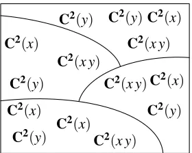
In its third configuration, our system employs clustering techniques in order to exploit semantic differences that may naturally emerge from each context in which the collocation and its constituents are used. Different senses of a collocation might have different compositionality measures as can be seen in these two example sentences employing the collocationgreat deal:

1. Two cans of soup for the price of one is such a

great deal!

C2(y) C2(y)C2_(x) C2(x y)

C2(x)

C2(x y)

C2(y)

C2(y)

C2(x)

C2(x y)

C2(x)

C2_(x) C2(y) _C2_{(x y)}

Figure 1: Example of a clustered second-order context vector space.

2. The tsunami caused agreat dealof damage to the country’s infrastructure.

In Word Sense Induction, clustering is used to group occurrences of a target word according to its sense or usage in context (see e.g. Pedersen (2010)) as it is expected that each cluster will represent a different sense or usage of the target word. However, since the contexts that human annotators referred to when judging the compositionality of the collocations was not provided, our system employs a workaround that uses a weighted average when measuring composi-tionality. This workaround is explained in what fol-lows.

In this configuration, the system first builds word vectors for the 20,000 most frequent words in the corpus (equation 2), and then uses these to compute the second-order context vectors for each occurrence of the collocation and its constituents in the corpus (equation 3). After context vectors for all occur-rences have been computed, they are clustered using CLUTO’s repeated bisections algorithm2. The vec-tors are clustered across a small numberKof clus-ters (we employedK=4). We expect that each clus-ter will represent a different contextual usage of the collocation, its headword and its modifier. Figure 1 depicts how a context vector space could be parti-tioned withK=4.

The system then for each clusterkbuilds the word vectors (equation 2)Wk(x y),Wk(x), andWk(y)for

the collocation, its headword and its modifier, from the contexts grouped within the clusterk. The com-positionality measure for the third configuration is then basically a weighted average over the clusters

of thec1score using each cluster, that is:

c₃=

K

∑

kkk

N

1 2

cos(Wk(x y),Wk(x))

+cos(Wk(x y),Wk(y))

(9)

wherekkkis the number of contexts in cluster k

andNis the total number of contexts across all clus-ters.

For all three configurations, the value reported as the numeric compositionality score was the corre-sponding value obtained from equations (5), (8) or (9), multiplied by 100. Each configuration’s nu-meric scores ci were binned into the three coarse

compositionality classes by comparing them with the configuration’s maximum value through equa-tion (10).

coarse(ci) =



 

 

high if2₃max≤ci

medium if1₃max<ci<2₃max

low ifci≤1₃max

(10)

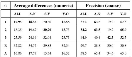
4 Results and conclusion

Table 1 shows the evaluation results for the three system configurations and two baselines. The left-hand side of the table shows the average difference between the gold-standard numeric score and each configuration’s numeric score. The right-hand side reports the precision on binning the numeric scores into the coarse classes. Evaluation scores are re-ported on all collocations and on the collocation sub-types separately. RowR is the baseline suggested by the workshop organisers, assigning random nu-meric scores, in turn binned into the coarse cate-gories. Row A shows the performance of a con-stant output baseline, assigning all collocations the

meangold-standard numeric score from the training set: 66.45, and then applying the binning strategy of equation (10) to this – which always assigns the coarse categoryhigh.

The first thing to note from this table is that con-figurations 1 and 2 generally outperform configu-ration 3, both on the mean difference and coarse scores. Configuration 1 slightly outperforms con-figuration 2 on the mean numeric difference scores, whilst configuration 2 is very close to and slightly

C Average differences (numeric) Precision (coarse)

ALL A-N S-V V-O ALL A-N S-V V-O

1 17.95 18.56 20.80 15.58 53.4 63.5 19.2 62.5

2 18.35 19.62 20.20 15.73 54.2 63.5 19.2 65.0 3 25.59 24.16 32.04 23.73 44.9 40.4 42.3 52.5

R 32.82 34.57 29.83 32.34 29.7 28.8 30.0 30.8

A 16.86 17.73 15.54 16.52 58.5 65.4 34.6 65.0

Table 1:Evaluation results of the three system configura-tions and two baselines on the test dataset. Best system scores on each grammatical subtype highlighted in bold.

better than configuration 1 on the coarse precision scores. The exception is that configuration 3 was the best performer on the coarse precision scoring for theS-Vsubtype.

The R baseline is outperformed by configurations 1, 2 and 3; roughly speaking where 1 and 2 out-perform R byd, configuration 3 outperforms R by aroundd/2. The A baseline generally outperforms all our system configurations. It seems to be also a quite competitive baseline for other systems partici-pating in the shared task.

The other trend apparent from the table is that per-formance on theV-OandA-Nsubtypes tends to ex-ceed that on the theS-Vsubtype.

An examination of the gold standard test files shows that the distribution over the

low/medium/high categories is similar for both

V-OandA-N, in both cases close to 0.08/0.27/0.65, with high covering nearly two-thirds of cases, whilst for S-V the distribution is quite different: 0.0/0.654/0.346, with medium covering nearly two-thirds of cases. This is reflected in the A baseline precision scores, as for each subtype these will necessarily be the proportion of gold-standard

high cases. This explains for example why the A baseline is much poorer on the S-V cases (34.6) than on the other cases (65.0, 65.4).

P

ercent of T

otal

0 10 20 30

0 20 40 60 80 100

A−N Conf 1

S−V Conf 1

0 20 40 60 80 100

V−O Conf 1 A−N

Test GS

0 20 40 60 80 100

S−V Test GS

0 10 20 30

V−O Test GS

Figure 2: The distribution of the gold standard numeric score vs. the distribution of the system’s first configura-tion numeric scores.

A-N S-V V-O

Instances 177254 11092 121317

Avg intervening 0.0684 0.3867 0.4612

Table 2: Some corpus statistics: the number of matched collocations per subtype (Instances) and the average number of intervening words per subtype (Avg interven-ing).

the contrast in the distributions seems broadly con-sistent with the mean numeric difference scores of Table 1.

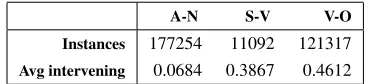
One can speculate on the reasons for the system’s poorer performance on the S-V subtype. The sys-tem treats intervening words in a collocation in a particular way, namely by ignoring them. This is one option, and another would be to include them as features counted in the vectors. Table 2 shows the average intervening words in the occurrences of the collocations. S-VandV-O are alike in this respect, both being much more likely to present intervening words than collocations of theA-Nsubtype. So the explanation of the poorer performance onS-V can-not lie there. Also because the average number of intervening words is low, we believe it is unlikely that including them as features will impact perfor-mance significantly.

Table 2 also gives the number of matched collo-cations per subtype. The number for theS-V collo-cations is an order of magnitude smaller than for the other subtypes. Although the collocations supplied by the organisers are in their base form, the system attempts to match them ’as is’ in the unlemmatised

version of the corpus. Whilst forA-NandV-O the base-form sequences relatively frequently do double service as inflected forms, this is far less frequently the case for the S-V sequences (e.g. user see ( S-V) is far less common than make money (V-O) ). This much smaller number of occurrences forS-V

cases, or the fact that they are drawn from syntac-tically special contexts, may be a factor in the rel-atively poorer performance. This perhaps is also a factor in the earlier noted fact that although config-uration 3 was generally outperformed, on theS-V

subtype the reverse occurs.

The unlemmatised version of the corpus was used because initial experimentation with the validation set produced slightly better results when employing raw words as features rather than lemmas. A possi-bility for future work would be to to refer to lemmas for matching collocations in the corpus, but to con-tinue to use unlemmatised words as features.

Other areas for future investigation involve the ef-fects of weighting schemes (such as IDF) and the use of similarity measures other than cosine, as well as alternatives in configurations 2 and 3. For example, configuration 2 could involve the modifier in the computation of the compositionality score, and configuration 3 could create separate clustering spaces for collocation, headword and modifier and compute similarity scores based on vectors represen-ting these clusters.

In sum, the simplest configuration of a totally un-supervised system yielded surprisingly good results at measuring compositionality of collocations in raw corpora, and whereas there is scope for further de-velopment and refinement, the system as it is consti-tutes a robust baseline to compare against more ela-borate systems.

5 Acknowledgements

References

Marco Baroni, Silvia Bernardini, Adriano Ferraresi, and Eros Zanchetta. 2009. The WaCky wide web: a collection of very large linguistically processed web-crawled corpora. Language Resources and Evalua-tion, 43(3):209–226, February.

Chris Biemann and Eugenie Giesbrecht. 2011. Distribu-tional Semantics and ComposiDistribu-tionality 2011: Shared Task Description and Results. InProceedings of the Distributional Semantics and Compositionality work-shop (DISCo 2011) in conjunction with ACL 2011, Portland, Oregon.

Diana McCarthy, Bill Keller, and John Carroll. 2003. Detecting a continuum of compositionality in phra-sal verbs. InProceedings of the ACL 2003 workshop on Multiword expressions: analysis, acquisition and treatment-Volume 18, pages 73–80, Sapporo. Associa-tion for ComputaAssocia-tional Linguistics.

Ted Pedersen. 2010. Duluth-WSI: SenseClusters applied to the sense induction task of SemEval-2. In Procee-dings of the 5th International Workshop on Seman-tic Evaluation, number July, pages 363–366, Uppsala, Sweden. Association for Computational Linguistics. Amruta Purandare and Ted Pedersen. 2004. Word

sense discrimination by clustering contexts in vector and similarity spaces. Proceedings of the Conference on Computational Natural Language Learning, pages 41–48.