GAMBL, genetic algorithm optimization of memory based WSD

GAMBL, Genetic Algorithm Optimization of Memory-Based WSD

Bart Decadt and V´eronique Hoste and Walter Daelemans

CNTS – Language Technology Group – University of Antwerp Universiteitsplein 1 – 2610 Wilrijk – Belgium

{bart.decadt,veronique.hoste,walter.daelemans}@ua.ac.be

Antal van den Bosch

Computational Linguistics – ILK – Tilburg University P.O. Box 90153 – 5000 LE Tilburg – The Netherlands

[email protected]

Abstract

GAMBL is a word expert approach to WSD in which each word expert is trained using memory-based learning. Joint feature selection and algo-rithm parameter optimization are achieved with a genetic algorithm (GA). We use a cascaded classi-fier approach in which the GA optimizes local con-text features and the output of a separate keyword classifier (rather than also optimizing the keyword features together with the local context features). A further innovation on earlier versions of memory-based WSD is the use of grammatical relation and chunk features. This paper presents the architecture of the system briefly, and discusses its performance on the English lexical sample and all words tasks in SENSEVAL-3.

1 Memory-Based WSD

We interpret WSD as a classification task distributed over word experts: given an ambiguous word and its context as input features, a classifier specialized on that word assigns the contextually appropriate sense to it. For each word-lemma–POS-tag combi-nation, a separate classifier is trained. Information about the words immediately surrounding the am-biguous word (the local context), as well as infor-mation about sense-related words in a wider context (keywords) are provided as information sources, coded in a feature vector. To train the word ex-perts, memory-based learning (MBL) is used, an in-stance of the lazy learning paradigm: all contexts in which an ambiguous word occurs in the training text are kept in memory and abstraction only occurs at classification time by extrapolating a class from the most similar item(s) in memory to the new test item. This contrasts with eager learning methods such as decision lists which abstract from the training data at training time and forget about the examples them-selves. For our experiments, we use the MBL al-gorithms implemented in TIMBL1. This software

1_{We used}

TIMBL version 5.0.0, which is available from

http://ilk.kub.nl

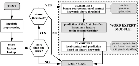
Figure 1: An overview of our architecture for word sense disambiguation.

YES

NO

is sent as a feature to the second classifier

CLASSIFIER 2

based on binary keywords local context and prediction

CLASSIFIER 1

binary representation of context

TEXT

WORD EXPERT MODULE

ASSIGN SENSE

linguistic preprocessing

lookup lexicon sense

above threshold?

YES NO

prediction of the first classifier keywords above threshold

parameter optimization and feature selection with genetic algorithm

heuristic

optimization parameter

than one sense?

more

allows a choice between different statistical and information-theoretic feature and value weighting methods, different neighborhood size and weighting parameters, etc., that should be optimized for each word expert independently. See (Daelemans et al., 2003b) for more information. It has been claimed, e.g. in (Daelemans et al., 1999), that lazy learn-ing has the right bias for learnlearn-ing natural language processing tasks as it makes possible learning from atypical and low-frequency events that are usually discarded by eager learning methods.

Architecture. Previous work on memory-based

WSD includes work from Ng and Lee (1996), Veen-stra et al. (2000), Hoste et al. (2002) and Mihalcea (2002). The current design of our WSD system is largely based on Hoste et al. (2002).

Figure 1 gives an overview of the design of our WSD system: the training text is first linguistically analyzed. For each word-lemma–POS-tag combi-nation, we check if it (i) is in our sense lexicon, (ii) has more than one sense and (iii) has a frequency in the training text above a certain threshold. For all combinations matching these three conditions, we train a word expert module. To all combinations with only one sense, or with more senses and a fre-quency below the threshold, we assign the default sense, which is respectively the only or most fre-quent sense in WordNet.

The word expert module consists of two cascaded memory-based classifiers: the sense predicted by

the first classifier is used as a feature in the second classifier. The first classifier is trained on keywords selected according to a statistical criterion, and the second one is trained on the prediction of the first and on the local context of the ambiguous word-lemma–POS-tag combination.

In the remainder of this paper, we will describe the feature construction process from the available information sources (Section 2), the learning and optimization approach (Section 3), and the results (Section 4) and their interpretation.

2 Information sources

Preprocessing. The training corpus is a

concate-nation of various sense-tagged English texts: it con-tains SemCor (included with WordNet 1.7.1), train-ing and test data from the English lexical sam-ple (LS) and all words (AW) tasks from previous SENSEVAL workshops, the line-, hard- and serve-corpora, and the example sentences in WordNet 1.7.1. This corpus contains 4.494.909 tokens of which 555.269 are sense-tagged words.

To this corpus, we add the training data from theSENSEVAL-3 English LS task, containing 7860 sense-tagged words. For the AW task, we sim-ply append the LS training data after conversion of the verb’s WordSmyth senses to WordNet 1.7.1 senses. For the LS task, however, we slightly change the design of the word expert module be-cause (i) WordSmyth senses are used for the verbs, and (ii) for some words in the LS task, the sense dis-tribution in our own training corpus is very different from the distribution in the LS training data – we did not want this difference to (heavily) influence the results.

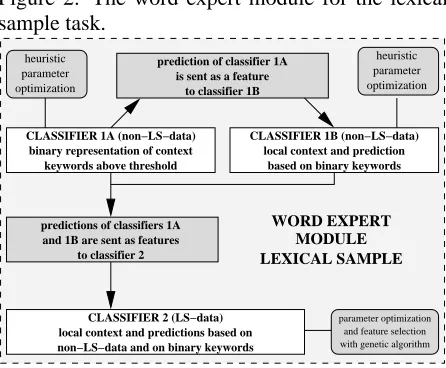
Figure 2 shows the word expert module used in the LS task: we first generate a sense prediction us-ing classifier 1A, trained on our own trainus-ing data using context keywords as features. This predic-tion becomes an extra feature in classifier 1B, also trained on our own training data but using local con-text as information source. Finally, the predictions of classifiers 1A and 1B become extra features for classifier 2: this classifier is trained on the LS train-ing data, and uses local context for disambiguattrain-ing senses.

The test data in the English LS task contains 3944 words to be sense-tagged (57 unique word-lemma– POS-tag combinations), and in the English AW task 2041 words (1020 combinations). Training and test data are linguistically analyzed: first, we tokenize, POS-tag, and find chunks and grammatical relations in the data with a shallow parser, and then we lem-matize the data. These tools were developed locally.

Figure 2: The word expert module for the lexical sample task.

parameter optimization and feature selection with genetic algorithm

WORD EXPERT MODULE LEXICAL SAMPLE

keywords above threshold

to classifier 2

prediction of classifier 1A is sent as a feature

to classifier 1B

predictions of classifiers 1A

CLASSIFIER 2 (LS−data) local context and predictions based on non−LS−data and on binary keywords binary representation of context CLASSIFIER 1A (non−LS−data)

local context and prediction based on binary keywords CLASSIFIER 1B (non−LS−data)

and 1B are sent as features

optimization heuristic parameter

heuristic

optimization parameter

In our training data we find 3433 word-lemma– POS-tag combinations that fulfilled the word expert criteria: in the LS test data, these word experts cover all 57 word-lemma–POS-tag combinations, and in the AW test data, they cover 596 combinations, or 1448 particular instances (70.95%).

We will continue with a description of how we create local context feature vectors, and extract key-words to create binary feature vectors.

Local context. The second classifier uses the

im-mediate local context of a focus word-lemma–POS-tag combination to disambiguate its senses: the fo-cus word itself, and the three words before and after it. For each of these seven words, we include in the feature vector the POS-tag and the chunk+relation-tag assigned to the word by the shallow parser. The chunk+relation-tag contains information on the ba-sic phrase type of the word (nominal, verbal, prepo-sitional), and for nominal phrases also information on the grammatical function (subject or object) of the phrase.

We set the context window size to±3 for prac-tical reasons: in the optimization step, we use a genetic algorithm for feature selection. This algo-rithm will determine which features from the con-text window will eventually be used in the classifi-cation step. Increasing the initial context window size, however, also increases the amount of com-puter time needed for the optimization step. Using a larger context window was computationally not fea-sible.

Keywords in context. The first classifier of each word expert is trained on information about possi-ble disambiguating keywords in a context of three sentences: the sentence in which the ambiguous word occurs, the previous sentence, and the follow-ing sentence. The method we use to extract the key-words for each sense is based on the work of Ng and Lee (1996). They determine the probability of a sensesof a focus lemmafgiven keywordkby di-vidingNs,kloc(the number of occurrences of a

pos-sible local context keywordkwith a particular focus word-lemma–POS-tag combinationwwith a partic-ular sense s) by Nkloc (the number of occurrences

of a possible local context keywordklocwith a par-ticular focus word-lemma–POS-tag combinationw regardless of its sense). In addition, we also take into account the frequency of a possible keyword in the complete training corpusNkcorp:

p(s|k) = Ns,kloc Nkloc ×(

1

Nkcorp) (1)

Words were selected as keywords for a sense if (i) they appeared at least three times in the context of that sense, and (ii)p(s|k)was higher than or equal to 0.001.

To this collection of local context keywords we add possible disambiguating content words ex-tracted from the WordNet sense definitions for each focus word-lemma–POS-tag combination. All the keywords are represented as binary features, of which the value is 1 if the keyword is present in the three-sentence-context, and 0 if not.

For each training item in the word experts, we generate a keyword-based prediction. First, we split the complete set of training items for each word ex-pert in ten folds of equal size. We then use nine folds to predict the sense of the remaining fold, af-ter having found an optimal parameaf-ter setting for TIMBLwith heuristic optimization on the nine folds. We repeat this procedure for each fold. Finally, for each training item, we append its keyword-based prediction to the local context feature vector.

3 Training and optimization

In previous work on memory-based WSD (Veenstra et al., 2000; Hoste et al., 2002) we showed that op-timization of features and algorithm parameters for each word expert independently contributes consid-erably to accuracy. For classifier 1 in the AW task, and for classifiers 1A and 1B in the LS task, we heuristically determine the optimal algorithm pa-rameter settings: we exhaustively try out all pos-sible combinations of (a selection of) distance met-rics, feature-weightings, number of nearest

neigh-bors and nearest neighbor voting schemes, and re-tain the best result. The testing of one setting is done with ten-fold cross-validation.

For classifier 2, we use a genetic algorithm (GA, e.g. (Goldberg, 1989)) to do joint parameter opti-mization and feature selection. We refer to (Daele-mans et al., 2003a) for a discussion of the effect of joint parameter optimization and feature selec-tion on accuracy of classifiers for NLP tasks. Joint feature selection and parameter optimization is an optimization problem which involves searching the space of all possible feature subsets and parame-ter settings to identify the combination that is op-timal or near-opop-timal. Since exhaustive search in large search spaces is computationally not feasi-ble in practice, a GA is a more realistic approach to search the space. Contrary to traditional hill-climbing approaches, such as backward selection, the GA explores different areas of the search space in parallel.

For the experiments we use a generational GA implemented in the DeGA (Distributed Evaluation

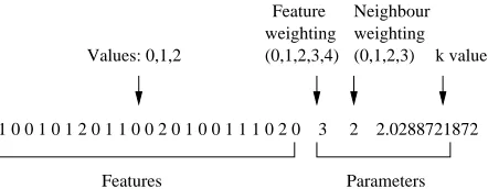
Genetic Algorithm) framework 2. We use the GA in its default settings. The GA optimization is per-formed using 10-fold cross-validation on the avail-able training data. The resulting optimal settings are then applied to the test data. In the experiments, the individuals are represented as bit strings (Fig-ure 3). Each individual contains particular values for all algorithm settings and for the selection of the features. ForTIMBL, the large majority of these fea-tures control the use of a feature (ignore, or a dis-tance metric) and are encoded in the chromosome as ternary alleles. At the end of the chromosome, the 5-valued weighting parameter and the 4-valued neighbor weighting parameter are encoded, together with thekparameter which controls the number of neighbors. The latter is encoded as a real value which represents the logarithm of the number of neighbors.

We will now present the results of our WSD ar-chitecture on the LS and AW test sets.

4 Experimental results

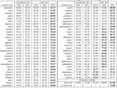
English lexical sample task. Table 1 presents the

results of our WSD system for each word in the LS task, and our overall score (the opt column). We included the results of TIMBL with default set-tings (the def column) and the score of a statistical baseline (the maj column), which assigns the sense

2

We would like to thank Bart Naudts for developing the DeGA environment, and adding TIMBL to this environment. More information on DeGA can be found at:

Figure 3: Example individual representing one TIMBLexperiment.

1 0 0 1 0 1 2 0 1 1 0 0 2 0 1 0 0 1 1 1 0 2 0 3 2 2.0288721872

Features

Values: 0,1,2 (0,1,2,3,4) weighting Feature

(0,1,2,3) weighting Neighbour

k value

Parameters

with the highest frequency in the training set to the test instances. For comparison, we also list ten-fold cross-validation results (with default and optimized settings) of the second classifier on the training set.

Looking at the overall score, we see that TIMBL with default settings already outperforms the base-line with 5%, and that the TIMBL classifier opti-mized with the GA, improves our score even more with another 7%.

For most words, the improvement after optimiza-tion with the genetic algorithm on the training set, also holds on the test set, though for 15 words, the optimal setting from the GA does not result in a bet-ter score than the default score. For four words, TIMBL and the GA cannot outperform the major-ity sense baseline. We do not yet know what causes TIMBL and the GA to perform badly, but a differ-ence between the sense distributions in the training and test set might be a factor. The distribution of the majority sense in the training set of source is 48.4%, while in the test set this distribution increases to 62.6%. For important there is a similar increase: from 38.9% to 47.4%. However, sense distribution differences in training and test set cannot be the only cause, because for activate and lose there is no such difference between the sense distributions.

Finally, Table 2 depicts the fine-grained classifi-cation accuracies of our system per POS in the LS task, again compared with the accuracies of the ma-jority sense baseline and TIMBL with default set-tings. The classification accuracy for nouns and verbs is more or less the same as the overall score. Adjectives, however, seem to be the harder to clas-sify for our system: the classification accuracy is 13% lower than the overall score. This could be re-lated to the on average higher number of senses for the adjectives.

English all words task. The last column of

Ta-ble 3 presents our results on the AW test set: the results of the classifier optimized with the GA are compared with the results of TIMBL with default settings, and with a majority sense baseline, which

Table 2: Classification accuracy per POS in the En-glish lexical sample task.

POS AVG. SENSES MAJ DEF OPT adjectives 7.4 51.6 50.3 54.1

nouns 6.0 54.2 56.9 66.4

verbs 5.6 56.5 64.3 69.4

Table 3: Classification accuracy in the English all words task.

TRAINING TEST WORD EXPERT WORDS

WordNet default / 56.4 TIMBL default 60.89 55.7 GA optimized TIMBL 72.50 60.1

ALL WORDS

WordNet default / 62.4

TIMBL default / 62.0

GA optimized TIMBL / 65.2

predicts for each word to be sense-tagged the sense that is listed in WordNet as the most frequent one. The first half of the table lists the results when we only take into account words for which a word ex-pert is built. TIMBL with default settings cannot outperform the already strong baseline, but after optimization with the GA, we see a 4% improve-ment. Unfortunately, this increase is not as high as the performance boost we see in the ten-fold cross-validation results on the training set, listed in the first column of Table 3: there is a large increase of 12% after the optimization step.

Words for which no word expert is built are tagged with their majority sense from WordNet. When we also take these words into account, we see similar results: again, defaultTIMBLcannot outper-form the baseline, but GA optimization gives a 3% increase.

5 Conclusion

From previous research on memory-based WSD, we learned that both feature selection, algorithm pa-rameter settings, and their interaction, play an im-portant role in accuracy, and that good selections and settings do not generalize over different word experts. These should therefore be optimized indi-vidually. We showed in this paper that using Ge-netic Algorithms andTIMBL, this complex multiple optimization problem can nevertheless be achieved, even for the AW task in which 3433 word experts have to be optimized.

in-Table 1: Classification accuracies for all lemmas in the English lexical sample task.

TRAINING SET TEST SET TRAINING SET TEST SET LEMMA/POS DEF OPT MAJ DEF OPT LEMMA/POS DEF OPT MAJ DEF OPT

provide/v 84.56 94.85 85.50 88.40 92.75 rule/n 75.44 91.23 40.00 50.00 60.00

eat/v 79.04 89.22 88.50 78.16 91.95 image/n 49.00 62.69 36.48 48.64 56.75

remain/v 85.40 95.62 78.57 82.85 88.57 paper/n 37.95 54.46 25.64 38.46 55.55

arm/n 88.67 93.20 81.95 84.21 84.96 produce/v 50.54 65.22 52.12 53.19 55.31

plan/v 67.93 78.48 82.14 75.00 83.33 suspend/v 46.34 59.35 35.93 34.37 51.56

add/v 73.95 82.38 46.21 79.54 82.57 argument/n 42.04 57.58 51.35 43.24 51.35

degree/n 64.56 78.38 60.93 71.09 82.03 difficulty/n 35.48 58.06 17.39 34.78 39.13

hot/a 68.67 78.00 79.06 76.74 81.39 performance/n 38.21 52.85 26.43 28.73 39.08

watch/v 85.71 89.80 74.50 78.43 80.39 use/v 80.77 88.46 71.42 78.57 78.57

smell/v 70.41 85.27 40.00 74.54 78.18 hear/v 64.52 74.19 46.87 53.12 53.12

bank/n 61.36 79.22 67.42 59.84 78.03 win/v 50.65 68.83 43.58 48.71 48.71

expect/v 64.93 77.92 74.35 73.07 76.92 different/a 54.81 65.27 50.00 46.00 46.00

talk/v 77.37 83.21 72.60 73.97 75.34 miss/v 40.00 68.89 33.33 43.33 43.33

appear/v 79.24 87.17 44.36 71.42 75.18 solid/a 9.80 31.78 31.03 27.58 27.58

decide/v 72.95 86.89 67.74 70.96 74.19 receive/v 75.00 80.77 88.88 92.59 88.88

wash/v 32.26 62.90 67.64 52.94 73.52 mean/v 84.81 91.14 52.50 77.50 75.00

organization/n 67.66 77.51 73.21 69.64 73.21 audience/n 73.90 85.29 67.00 76.00 74.00

party/n 61.82 71.96 62.06 65.51 72.41 operate/v 72.73 84.85 38.88 66.66 55.55

interest/n 63.28 70.36 41.93 59.13 72.04 write/v 64.29 71.43 34.78 56.52 43.47

express/v 48.62 72.48 69.09 45.45 70.90 play/v 48.42 64.21 46.15 51.92 42.30

sort/v 61.09 78.60 65.62 66.66 70.83 difference/n 57.14 68.51 40.35 47.36 46.49

atmosphere/n 47.42 60.20 66.66 51.85 70.37 judgment/n 35.64 60.40 28.12 40.62 34.37

note/v 56.15 69.23 56.71 61.19 68.65 treat/v 37.84 55.86 28.07 40.35 38.59

disc/n 54.03 69.19 38.00 52.00 66.00 lose/v 44.78 62.69 52.77 36.11 52.77

climb/v 63.48 78.26 55.22 59.70 64.17 important/a 72.08 82.23 47.36 42.10 47.36

shelter/n 66.14 74.02 44.89 54.08 63.26 activate/v 70.40 80.27 82.45 64.91 80.70

simple/a 43.55 58.52 27.77 44.44 61.11 source/n 34.06 52.90 65.62 46.87 59.37

ask/v 49.80 62.06 28.24 60.30 61.06 OVERALL SCORE

begin/v 53.41 63.07 59.49 53.16 60.75 FINE-GR. 59.82 71.28 55.22 60.80 67.40

encounter/v 51.94 65.89 36.92 58.46 60.00 COARSE-GR. / / / / 74.00

Table 4: The GA’s selection of the different types of features in percentages.

PREDICTION TYPE AW LS predictions from keyword classifier 59 74 predictions from old data classifier / 65 words in local context 59 58 POS-tags of local context 55 65 chunk+relation tags of local context 67 72

formation seems to contribute to the disambiguation process: Table 4 list for each type of feature the per-centage of times it was selected by the GA. Though Table 4 is an not exhaustive comparison of the dif-ferent types of features, we nevertheless see that the GA selects syntactic and grammatical information more often than plain words or POS-tags.

Finally, Table 4 also suggests that our cascaded approach to combine two different information sources is quite successful: the predictions from the previous classifier(s) are very often selected, espe-cially in the LS task, where the prediction from the keyword classifier is most often selected.

References

W. Daelemans, A. van den Bosch, and J. Zavrel. 1999. Forgetting exceptions is harmful in

lan-guage learning. Machine Learning, 34:11–43. W. Daelemans, V. Hoste, F. De Meulder, and

B. Naudts. 2003a. Combined optimization of feature selection and algorithm parameter inter-action in machine learning of language. In Proc.

of ECML-2003, pages 84–95.

W. Daelemans, J. Zavrel, K. van der Sloot, and A. van den Bosch. 2003b. TiMBL: Tilburg memory-based learner, ver. 5.0, ref. guide. Tech. report, ILK.

D. Goldberg. 1989. Genetic Algorithms in Search,

Optimization and Machine Learning. Addison

Wesley.

V. Hoste, I. Hendrickx, W. Daelemans, and A. van den Bosch. 2002. Parameter optimization for machine-learning of word sense disambigua-tion. Nat. Language Eng., 8:311–325.

Rada Mihalcea. 2002. Instance based learning with automatic feature selection applied to word sense disambiguation. In Proc. of COLING-2002. H. T. Ng and H. B. Lee. 1996. Integrating multiple

knowledge sources to disambiguate word senses: An examplar-based approach. In Proc. of

ACL-1996, pages 40–47.