Dynamic Feature Induction:
The Last Gist to the State-of-the-Art
Jinho D. Choi
Department of Mathematics and Computer Science Emory University
Atlanta, GA 30322, USA
Abstract
We introduce a novel technique called dynamic feature induction that keeps inducing high di-mensional features automatically until the fea-ture space becomes ‘more’ linearly separable. Dynamic feature induction searches for the fea-ture combinations that give strong clues for distinguishing certain label pairs, and gener-ates joint features from these combinations. These induced features are trained along with the primitive low dimensional features. Our ap-proach was evaluated on two core NLP tasks, part-of-speech tagging and named entity recog-nition, and showed the state-of-the-art results for both tasks, achieving the accuracy of97.64 and the F1-score of91.00respectively, with about a 25% increase in the feature space.
1 Introduction
Feature engineering typically involves two processes: the process of discovering novel features with domain knowledge, and the process of optimizing combina-tions between existing features. Discovering novel features may require linguistic background as well as good understanding in machine learning such that it is often difficult to do. Optimizing feature combi-nations can be also difficult but usually requires less domain knowledge and more importantly, it can be as effective as discovering new features. It has been shown for many tasks that approaches using simple machine learning with extensive feature engineering outperform ones using more advanced machine learn-ing with less intensive feature engineerlearn-ing (Xue and Palmer, 2004; Bengtson and Roth, 2008; Ratinov and Roth, 2009; Zhang and Nivre, 2011).
Recently, people have tried to automate the second part of feature engineering, the optimization of fea-ture combinations, through leading-edge models such as neural networks (Collobert et al., 2011). Coupled with embedding approaches (Mikolov et al., 2013; Le and Mikolov, 2014; Pennington et al., 2014), neural networks can find the optimal feature combinations using techniques such as random weight initialization and back-propagation, and have established the new state-of-the-art for several tasks (Socher et al., 2013; Devlin et al., 2014; Yu et al., 2014). However, neural networks are not as good at optimizing combinations between sparse features, which are still the most dom-inating factors in natural language processing.
This paper introduces a new technique called dy-namic feature induction that automates the optimiza-tion of feature combinaoptimiza-tions (Secoptimiza-tion 3), and can be easily adapted to any NLP task using sparse features. Dynamic feature induction allows humans to focus on the first part of feature engineering, the discovery of novel features, while machines handle the second part. Our approach was experimented with two core NLP tasks, part-of-speech tagging (Section 4) and named entity recognition (Section 5) and showed the state-of-the-art results for both tasks.
2 Background
2.1 Nonlinearity in NLP
Linear classification algorithms such as Perceptron, Winnow, or Support Vector Machines with a linear kernel have performed exceptionally well for various NLP tasks (Collins, 2002; Zhang and Johnson, 2003; Pradhan et al., 2005). This is not because our feature space is linearly separable by nature, but sparse
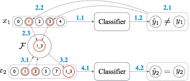
Figure 1:Overview of dynamic feature induction.
tures introduced to NLP yield very high dimensional vector space such that it is rather forced to be linearly separable. For example, NLP features for a wordwi typically involve the word forms ofwi−1andwi(e.g., fi−1,fi). If the feature space is not linearly separable with these features, a common trick is to introduce ‘higher’ dimension features by joining ‘lower’
dimen-sion features together (e.g.,fi−1 fi). The more joint features we introduce, the higher chance we get for the feature space being linearly separable although these joint features can be very overfitted.
Let us define low dimensional features as the primi-tive features such asfi−1orfi, and high dimensional features as the joint features such asfi fi+1.1 Low dimensional features are well explored for most NLP tasks; it is the high dimensional features that are quite sensitive to specific tasks. Finding high dimensional features can be a manual intensive work and this is what dynamic feature induction intends to take over. 2.2 Related Work
Kudo and Matsumoto (2003) introduced the polyno-mial kernel expansion that explicitly enumerated the feature combinations. Our approach is distinguished because they used a frequency-based PrefixSpan al-gorithm (Pei et al., 2001) whereas we used the online learning weights for finding the feature combinations. Goldberg and Elhadad (2008) suggested an efficient algorithm for computing polynomial kernel SVMs by combining inverted indexing and kernel expansion. Their work is focused more on improving support vector machines whereas our work is generalized to any linear classification algorithm.
1The joint features tend to yield a much higher dimensional feature space than the primitive features.
Okanohara and Tsujii (2009) introduced an approach for generating feature combinations using`1 regular-ization and grafting (Perkins et al., 2003). Although we share similar ideas, their grafting algorithm starts with an empty feature set whereas ours starts with low dimensional features, and their correlation parame-tersαi,yare pre-computed whereas ours are dynami-cally determined. Strubell et al. (2015) suggested an algorithm that dynamically selected strong features during decoding. Our work is distinguished because we do not run multiple training phases as they do for figuring our strong features.
3 Dynamic Feature Induction
The intuition behind dynamic feature induction is to keep populating high dimensional features by joining low dimensional features together until the feature space becomes ‘more’ linearly separable.2 Figure 1
shows how features are induced during training: 1. Given a training instance(x1, y1), wherex1is a
feature set consisting of 5 features andy1is the gold label, the classifier predicts the labelyˆ1. 2. Let us refer “strong features foryagainstyˆ” to
features that give strong clues for distinguishing
yfromyˆ. Ifyˆ1 is not equal toy1(2.1), strong features fory1againstyˆ1inx1are selected (2.2), and combinations of these features are added to the induced feature setF (2.3).
3. Given a new training instance(x2, y2), combi-nations of features inx2are checked byF(3.1), and appended tox2if allowed (3.2).
4. The extended feature setx2is fed into the classi-fier. Ifyˆ2 is equal toy2, no feature combination is induced fromx2.
Thus, high dimensional features inFare incremen-tally induced and learned along with low dimensional features during training. During decoding, each fea-ture set is extended by the induced feafea-tures inF, and the prediction is made using the extended feature set. The size ofF can grow up to|X |2, where|X |is the size of low dimensional features. However, we found that|F|is more like1/4· |X |in practice.
The following sections explain our approach in de-tails. Sections 3.1, 3.2, and 3.3 describe how features are induced and learned during training. Sections 3.4 and 3.5 describe how the induced features are stored and expanded during decoding.
3.1 Feature Induction
Algorithm 1 shows an online learning algorithm that induces and learns high dimensional features during training. It takes the set of training instancesDand the learning rateη, and returns the weight vectorw and the set of induced featuresF.
Algorithm 1Feature Induction
Input: D: training set,η: learning rate.
Output: w: weight vector,F: induced feature set. 1: w←g←0
2: F ←∅
3: until max epoch is reached do
4: foreach (x, y)∈D do
5: yˆ←arg maxy0∈Y(w·φ(x, y0,F)−Iy(y0)) 6: if y6= ˆy then
7: ∂←φ(x, y,F)−φ(x,y,ˆ F) 8: g←g+∂◦∂
9: w←w+ (η/(ρ+√g))·∂
10: v←[w◦φ(x, y,∅)]y−[w◦φ(x,y,ˆ ∅)]yˆ
11: L ←argkmax∀ivi
12: for i= 2 to |L| do
13: F ← F ∪ {(L1,Li)}
14: return w,F
The algorithm begins by initializing the weight vector w, the diagonal vectorg, and the induced feature set F (lines 1-2). For each instance(x, y) ∈ Dwhere
y is the gold-label for the feature setx, it predicts ˆ
y maximizingw·φ(x, y0,F)−I
y(y0), whereI is defined as follows (lines 4-5):
Iy(y0)←
(
1, ify=y0.
0, otherwise.
The feature mapφtakes(x, y,F), and returns ad×l -dimensional vector, wheredand lare the sizes of features and labels, respectively; each dimension con-tains the value for a particular feature and a label.3
If certain combinations between features inxexist inF, they are appended to the feature vector along with the low dimensional features (see Section 3.5 for more details). The indicator functionIallows our algorithm to be optimized for the hinge loss for mul-ticlass classification (Crammer and Singer, 2002):
`h = max[0,1 +w·(φ(x,y,ˆ F)−φ(x, y,F))] Ifyis not equal toyˆ(line 6), the partial vector∂is measured (line 7), andgandware updated (lines 8-9) by AdaGrad (Duchi et al., 2011), where the learning rateηis adjusted byg(in our case,ρ=1E-5). Once wis updated, thed-dimensional vectorvis generated by subtracting[w◦φ(x,y,ˆ ∅)]ˆyfrom[w◦φ(x, y,∅)]y (line 10), where[. . .]yreturns only the portion of the values relevant toy(Figure 2).
The i’th element in v represents the strength of thei’th feature foryagainstyˆ; the greaterviis, the stronger thei’th feature is. Next, indices of the top-k
entries invare collected in the ordered listL(line 11), representing the strongest features foryagainstyˆ.4
Finally, the pairs of the first index inL, representing the strongest feature, and the other indices inLare added to the induced feature setF(lines 12-13). For example, ifL= [i, j, k]such thatvi≥vj ≥vk >0, two pairs,(i, j)and(i, k), are added toF.
For all our experiments,k= 3is used; increasing
kbeyond this cutoff did not show much improvement. Notice that all induced features inFare derived by joining only low dimensional features together. Our algorithm does not join a high dimensional feature with either a low dimensional feature or another high dimensional feature. This was done intentionally to prevent from the feature space being exploded; such features can be induced by replacing∅withFin the line 10 as follows:
v←[w◦φ(x, y,F)]y−[w◦φ(x,y,ˆ F)]yˆ 3In most cases, these values are either0or1.
Figure 2:Given the weight vectorwand the feature mapφ,[w◦φ(x, y,∅)]ytakes the Hadamard product betweenwandφ(x, y,∅), then truncates the resulting vector with respect to the labely.
It is worth mentioning that we did not find it useful for joining intermediate features together (e.g.,(j, k) in the above example). It is possible to utilize these combinations by weighting them differently, which we will explore in the future. Additionally, we exper-imented with the combinations between strong and weak features (joiningi’th andj’th features, where vi >0andvj <0), which again was not so useful. We are planning to evaluate our approach on more tasks and data, which will give us better understand-ing of what combinations are the most effective. 3.2 Regularized Dual Averaging
Each high dimensional feature inF is induced for making classification between two labels, yandyˆ, but it may or may not be helpful for distinguishing labels other than those two. Our algorithm can be modified to learn the weights of the induced features only for their relevant labels by adding the label in-formation toF, which would change the line 13 in Algorithm 1 as follows:
F ← F ∪ {(L1,Li, y,yˆ)}
However, introducing features targeting specific la-bel pairs potentially confuses the classifier, especially when they are trained with the low dimensional fea-tures targeting all labels. Instead, it is better to apply a feature selection technique such as`1 regulariza-tion so the induced features can be selectively learned for labels that find those features useful. We adapt regularized dual averaging (Xiao, 2010), which effi-ciently finds the convergence rates for online convex
optimization, and works most effectively with sparse feature vectors. To apply regularized dual averaging, the line 1 in Algorithm 1 is changed to:
w←g←c←0; t←1
cis ad×l-dimensional vector consisting of accu-mulative penalties.tis the number of weight vectors generated during training. Althoughwis technically not updated wheny= ˆy, it is still considered a new vector. Thus,tis incremented for every training in-stance, sot←t+ 1is inserted after the line 5.cis updated by adding the partial vector∂as follows (to be inserted after the line 7):
c←c+∂
Thus, each dimension increpresents the accumula-tive penalty (or reward) for a particular feature and a label. At last, the line 9 is changed to:
w←(η/(ρ+√g))·`1(c, t, λ)
`1(c, t, λ)← (
ci−sgn(ci)·λ·t, |c∀i|> λ·t.
0, otherwise.
3.3 Locally Optimal Learning to Search
Features in most NLP tasks are extracted from struc-tures (e.g., sequence, tree). For structured learning, we adapt “locally optimal learning to search” (Chang et al., 2015b), that is a member of imitation learning similar to DAGGER(Ross et al., 2011). LOLS not only performs well relative to the reference policy, but also can improve upon the reference policy, show-ing very good results for tasks such as part-of-speech tagging and dependency parsing. We adapt LOLS by setting the reference policy as follows:
1. The reference policyπdetermines how often the gold labelyis picked over the predicted labelyˆ to build a structure. For all our experiments,π
is initialized to0.95.
2. For the first epoch, sinceπis0.95,yis randomly picked overyˆfor 95% of the time.
3. After every epoch,πis multiplied by0.95. This allows the next epoch to pickyless often than the previous epoch (e.g.,π becomes0.952 = 0.9025for the 2nd epoch soyis picked about 90% of the time instead of 95%).
For our experiments, LOLS gave only marginal im-provement, probably because the tasks we evaluated, part-of-speech tagging and named entity recognition, did not yield complex structures. However, we still included this in our framework because we wanted to evaluate our approach on more tasks such as depen-dency parsing where learning to search algorithms show a clear advantage (Goldberg and Nivre, 2012; Choi and McCallum, 2013; Chang et al., 2015a). 3.4 Feature Hashing
Feature hashing is a technique of converting string features to vectors (Ganchev and Dredze, 2008; Wein-berger et al., 2009). Given a string featuref and a hash functionh, the index off in the vector space is determined by taking the remainder of the hash code:
k←hstring→int(f)modδ
The divisorδis tuned during development. Feature hashing allows to convert string features into sparse vectors without reserving an extra space for a map whose keys and values are the string features and their
indices. Given a feature index pair(i, j)representing strong features foryagainstyˆ(Section 3.1), the index of the induced feature can be measured as follows:
k←hint→int(i· |X |+j)modδ
For efficiency, feature hashing is adapted to our sys-tem such that the induced feature setFis actually not a set but aδ-dimensional boolean array, where each dimension represents the validity of the correspond-ing induced feature. Thus, the line 13 in Algorithm 1 is changed to:
k←hint→int(L1· |X |+Li)modδ
Fk←True
For the choice ofh, xxHashis used, that is a fast non-cryptographic hash algorithm showing the per-fect score on the Q.Score.5
3.5 Feature Expansion
Algorithm 2 describes how high dimensional features are expanded from low dimensional features during training and decoding. It takes the sparse vectorxl containing only low dimensional features and returns a new sparse vectorxl+h containing both low and high dimensional features.
Algorithm 2Feature Expansion
Input: xl: sparse feature vector containing only
low dimensional features.
Output: xl+h: sparse feature vector containing both
low and high dimensional features. 1: xl+h←copy(xl)
2: for i←1 to |xl| do
3: for j ←i+ 1 to |xl| do
4: k←hint→int(i· |X |+j)modδ
5: if Fk then xl+h.append(k)
6: return xl+h
The algorithm begins by copyingxltoxl+h (line 1). For every combination(i, j)∈xl×xl, whereiandj represent the corresponding feature indices (lines 2-3), it first measures the indexkof the feature com-bination (line 4), then checks if this comcom-bination is valid (Section 3.4). If the combination is valid, mean-ing that(Fk = True), kis added toxl+h (line 5). Finally,xl+h is returned with the expanded high di-mensional features.
4 Part-of-Speech Tagging 4.1 Corpus
The Wall Street Journal corpus from the Penn Tree-bank III is used (Marcus et al., 1993) with the stan-dard split for part-of-speech tagging experiments.
Set Sections Sentences ALL OOV
TRN 0-18 38,219 912,344 0
DEV 19-21 5,527 131,768 4,467 TST 22-24 5,462 129,654 3,649
Table 1:Distributions of the Wall Street Journal corpus.TRN: training,DEV: development,TST: evaluation, ALL: all words, OOV: out-of-vocabulary words.
4.2 Tagging and Learning Algorithms
A one-pass, left-to-right tagging algorithm is used for our experiments. Such a simple algorithm is chosen because we want to see the performance gain purely from our approach, not by a more sophisticated tag-ging algorithm (Toutanova et al., 2003; Shen et al., 2007), which may improve the performance further.
For learning, the final algorithm from Section 3 is used. Additionally, mini-batch is applied, where each batch consists of training instances fromk-number of sentences, causing the sizes of these batches different. We found that grouping instances with respect to the sentence boundary was more effective than batching them across arbitrary sentences. For all our experi-ments, the learning rateη= 0.02and the mini-batch boundaryk= 5were used without tuning.
4.3 Ambiguity Classes
The ambiguity class of a word is the concatenation of all possible tags for that word. For example, if the word ‘study’ can be tagged byNN(common noun) or VB(base verb), its ambiguity class becomesNN VB. Instead of building ambiguity classes only from the training dataset, we automatically tagged a mixture of large datasets, the English Wikipedia articles6and the
New York Times corpus,7and pre-constructed
ambi-guity classes using the automatic tags before training. This was motivated by Moore (2015), who showed extraordinary results on the out-of-vocabulary words by limiting the classification to the ambiguity classes collected from such large corpora.
6dumps.wikimedia.org/enwiki 7catalog.ldc.upenn.edu/LDC2008T19
We used the ClearNLP POS tagger (Choi and Palmer, 2012) for tagging the data (about 141M words), threw away tags appearing less than a certain threshold, and created the ambiguity classes. For each word, tags appearing less than 20% of the time for that word were discarded. As the result, about 2M ambiguity classes were collected from these datasets.
4.4 Feature Template
Table 2 shows the template for low dimensional fea-tures. Digits inside the curly brackets imply the con-text windows with respect to the wordwito be tagged. For example,f{0,±1} represents the word-forms of
wi,wi−1, andwi+1. No joint features (e.g.,f0 f1) are included in this template; they should be automat-ically induced by dynamic feature induction.
Orthographic (Gim´enez and M`arquez, 2004) and word shape (Finkel et al., 2005) features are adapted from the previous work. The positional features indi-cate whetherwiis the first or the last word in the sen-tence. Word clusters are trained on the same datasets in Section 4.3 using Brown et al. (1992).
f:{0,±1,±2}, fu:{0,±1,±2}, s:{0,±1}, c:{0,±1}, π2:{0}, π3:{0}, σ1:{0}, σ2:{0}, σ3:{0}, σ4:{0},
p:{0,−1,−2,−3}, a:{0,1,2,3},O:{0},P:{0}
Table 2:Feature template for part-of-speech tagging.f: word-form,fu: uncapitalized word-form,s: word shape,c: word cluster,πk:k’th prefix,σk:k’th suffix,p: part-of-speech tag,
a: ambiguity class,O: orthographic feature set,P: positional feature set.
4.5 Development
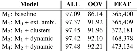
The regularization parameterλ(Section 3.2) and the modulo divisorδ(Section 3.4) are tuned during de-velopment through grid search onλ∈[1E-9, 1E-6] andδ ∈[1.5M, 5M]. Table 3 shows the accuracies achieved by our models on the development set.
[image:6.612.316.542.598.683.2]Model ALL OOV FEAT M0: baseline 97.09 86.14 365,400 M1: M0+ ext. ambi. 97.37 91.92 365,409 M2: M1+ clusters 97.45 91.96 372,181 M3: M1+ dynamic 97.42 92.10 468,378 M4: M2+ dynamic 97.48 92.21 473,134
M0used the tagging and the learning algorithms in Section 4.2 and the feature template in Section 4.4, where the ambiguity classes were collected only from the training dataset; dynamic feature induction was not used for M0. By applying the external ambiguity classes in Section 4.3, M1achieved about a 5.8% im-provement on OOV. M2gained small improvements by adding word clusters. Coupled with dynamic fea-ture induction, M3and M4gained about0.04% and 0.2% improvements on average for ALL and OOV.
For both M3 and M4, about 100K more features were generated from M1and M2, implying that about 25% of the features were automatically induced by dynamic feature induction. It is worth pointing out that improving upon M1 was a difficult task because it was already reaching near the state-of-the-art. The external ambiguity classes by themselves were strong enough to make accurate predictions such that the induced features did not find a critical role in the classification.
4.6 Evaluation
Table 4 shows the accuracies achieved by the models from Section 4.5 and the previous state-of-the-art approaches on the evaluation set.
Approach ALL OOV EXT Manning (2011) 97.29 89.70
Manning (2011) 97.32 90.79 X
Shen et al. (2007) 97.33 89.61
Sun (2014) 97.36
-Moore (2015) 97.36 91.09 X
Spoustov´a et al. (2009) 97.44 - X
Søgaard (2011) 97.50 - X
Tsuboi (2014) 97.51 91.64 X
This work: M0 97.18 86.35 This work: M1 97.37 91.34 X This work: M2 97.46 91.23 X This work: M3 97.52 91.53 X
This work: M4 97.64 92.03 X Table 4:Part-of-speech tagging accuracies on the evaluation set. EXT: whether or not the approach used external data.
The results on the evaluation set appear much more promising. Still, the biggest gain was made by M1, but our final model M4was able to achieve a 0.8% im-provement on OOV over M2, and showed the state-of-the-art results on both ALL and OOV. Interestingly,
M2showed a slightly lower accuracy on OOV than M1even with the additional word cluster features. On the other hand, M2 did show a slightly higher accu-racy on ALL, indicating that the model was probably too overfitted to the in-vocabulary words.8 However,
M4was still able to achieve improvements over M2 on both ALL and OOV, implying that dynamic fea-ture induction facilitated the classifier to be trained more robustly.
5 Named Entity Recognition 5.1 Corpus
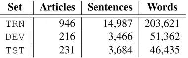
The English corpus from the CoNLL’03 shared task is used (Tjong Kim Sang and De Meulder, 2003) for named entity recognition experiments.
Set Articles Sentences Words
TRN 946 14,987 203,621
DEV 216 3,466 51,362
[image:7.612.333.523.282.341.2]TST 231 3,684 46,435
Table 5:Distributions of the English corpus from the CoNLL’03 shared task.TRN: training,DEV: development,TST: evaluation.
5.2 Feature Template
Table 6 shows the feature template for NER, adapting the specifications in Table 2. Following the state-of-the-art approaches (Table 8), word clusters are trained on the Reuters Corpus Volume I (Lewis et al., 2004) using Brown et al. (1992). Named entity gazetteers are collected from DBPedia.9 Word embeddings are
trained on the datasets in Section 4.3 using Mikolov et al. (2013) and appended to the sparse feature vec-tors as dense vecvec-tors. Note that the word embedding features did not participate in dynamic feature induc-tion; it was not intuitive how to combine sparse and dense features together so we left it as a future work.
f:{0,±1}, fu:{0,±1,±2}, s:{0,±1}, l:{0}, c:{0,1,2},
e:{0,±1,±2,±3,±4}, π1:{0}, π3:{1}, σ1:{0}, σ3:{−1,0}, p:{0,±1,±2}, n:{−1,−2,−3}, z:{±1,0,2,3},O:{0},O:{1}
Table 6:Feature template for named entity recognition.f: word-form,fu: uncapitalized word-form,s: word shape,l: lemma,
c: word cluster,e: word embedding,πk:k’th prefix,σk:k’th suffix,p: part-of-speech tag,n: named entity tag,z: named entity gazetteer,O: orthographic feature set.
8A similar trend is shown in Table 3 for M
5.3 Development
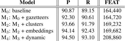
The regularization parameter and the modulo divisor are tuned during development through the same grid search in Section 4.5. Table 7 shows the precisions and the recalls achieved by our models on the devel-opment set (the F1-scores are shown in Table 8).
Model P R FEAT
M0: baseline 90.87 89.15 164,440
M1: M0+ gazetteers 92.30 90.61 164,720
M2: M1+ clusters 93.66 91.79 169,232
M3: M2+ embeddings 94.14 92.43 169,682
[image:8.612.78.297.160.233.2]M4: M3+ dynamic 94.50 93.10 208,860
Table 7:Precision and recall on the development set for named entity recognition. P: precision, R: recall.
M0used the tagging and the learning algorithms in Section 4.2 and the feature template in Section 5.2, excluding the gazetteer, cluster, and embedding fea-tures; dynamic feature induction was not applied to M0. M{1,2,3}gained incremental improvements from
the gazetteer, cluster, and embedding features, respec-tively. M4showed0.36% and0.67% improvements on precision and recall respectively, and generated about 40K more features compared to M3. This is about 23% increase in features that is similar to the increase shown in Table 3.
[image:8.612.82.288.488.641.2]5.4 Evaluation
Table 8 shows the F1-scores achieved by our models and the previous state-of-the-art approaches.10
Approach DEV TST Turian et al. (2010) 93.25 89.41 Suzuki and Isozaki (2008) 94.48 89.92 Ratinov and Roth (2009) 93.50 90.57 Lin and Wu (2009) - 90.90 Passos et al. (2014) 94.46 90.90 This work: M0 90.00 84.44 This work: M1 91.45 86.85 This work: M2 92.72 89.64 This work: M3 93.27 90.57 This work: M4 93.79 91.00
Table 8:F1-scores on the development and the evaluation sets for named entity recognition.
10Ratinov and Roth (2009) reported the F1-score of 90.80 on the evaluation set, but that model was trained on both the training and the development sets so not compared in this table.
All models showed improvements over their prede-cessors; the improvements made in TST were more dramatic than the ones made in DEV although they followed a very similar trend. Notice that M3, not us-ing dynamic feature induction, showed very similar scores to Ratinov and Roth (2009). This was not sur-prising because M3 adapted many features suggested by them, except for the non-local features.11
M4achieved about 0.5% improvements over M3, showing the state-of-the-art result on TST. Consid-ering that M3was already near state-of-the-art, this improvement was meaningful. It was interesting that Suzuki and Isozaki (2008) achieved the state-of-the-art result on DEV although their score on TST was much lower than the other approaches. This might be because features extracted from the huge external data they used were overfitted to DEV, but more thor-ough analysis needs to be done. On the other hand, Passos et al. (2014) achieved the near state-of-the-art result on DEV while it also got a very high score on TST by utilizing phrase embeddings, which we will look into in the future.
6 Conclusion
In this paper, we introduced a novel technique called dynamic feature induction that automatically induces high dimensional features so the feature space can be more linearly separable. Our approach was evaluated on two NLP tasks, part-of-speech tagging and named entity recognition, and showed the state-of-the-art results on both tasks. The improvements achieved by dynamic feature induction might not be statistically significant, but important because they gave the last gist to the state-of-the-art; without this last gist, our system would have not reached the bar.
It is worth mentioning that we also experimented with several feature templates including many joint features without applying dynamic feature induction. The results we got from these manually induced fea-tures were not any better (often worse) than the ones achieved by dynamic feature induction, which was very encouraging. In the future, we will experiment our approach on more NLP tasks such as dependency parsing and conference resolution where induced fea-tures should play a more critical role.
We concede that our approach is more empirically motivated than theoretically justified. For instance, the choice ofk(line 11) or the combination configu-ration forL(line 13) in Algorithm 1 are rather empir-ically derived. All the parameters are automatempir-ically tuned by running grid searches on the development sets (Sections 4.5 and 5.3); it would be intellectually intriguing to find a more principled way of adjusting these hyper-parameters than just brute-force search. The locally optimal learning to search is used to help structured learning although it gives a relatively smaller impact to the tasks involving sequence clas-sification such as part-of-speech tagging and named entity recognition. This framework is used because we plan to apply our approach on more structurally oriented tasks such as dependency parsing and AMR parsing. Our work is also related to feature group-ing, which has been shown to be beneficial in learn-ing high-dimensional data (Zhong and Kwok, 2011; Suzuki and Nagata, 2013). It will be interesting to compare our work to the previous work and see the strengths and weaknesses of our approach.
Acknowledgments
We gratefully acknowledge the support of the Yahoo Academic Career Enhancement Award, the IPsoft Development Enhancement Grant, the University Re-search Committee Award, and the Infosys ReRe-search Enhancement Grant. Any contents expressed in this material are those of the authors and do not necessar-ily reflect the views of these awards and grants.
References
Eric Bengtson and Dan Roth. 2008. Understanding the Value of Features for Coreference Resolution. In Pro-ceedings of the 2008 Conference on Empirical Methods
in Natural Language Processing, EMNLP’08, pages
294–303.
Peter F. Brown, Peter V. deSouza, Robert L. Mercer, Vin-cent J. Della Pietra, and Jenifer C. Lai. 1992. Class-based n-gram Models of Natural Language.
Computa-tional Linguistics, 18(4):467–480.
Kai-Wei Chang, He He, Hal Daum´e III, and John Lang-ford. 2015a. Learning to Search for Dependencies.
arXiv:1503.05615.
Kai-Wei Chang, Akshay Krishnamurthy, Alekh Agarwal, Hal Daume, and John Langford. 2015b. Learning to Search Better than Your Teacher. InProceedings of the
32nd International Conference on Machine Learning,
ICML’15, pages 2058–2066.
Jinho D. Choi and Andrew McCallum. 2013. Transition-based Dependency Parsing with Selectional Branching.
InProceedings of the 51st Annual Meeting of the
Asso-ciation for Computational Linguistics, ACL’13, pages
1052–1062.
Jinho D. Choi and Martha Palmer. 2012. Fast and Robust Part-of-Speech Tagging Using Dynamic Model Selec-tion. InProceedings of the 50th Annual Meeting of the
Association for Computational Linguistics, ACL’12,
pages 363–367.
Michael Collins. 2002. Discriminative Training Methods for Hidden Markov Models: Theory and Experiments with Perceptron Algorithms. InProceedings of the conference on Empirical methods in natural language
processing, EMNLP’02, pages 1–8.
Ronan Collobert, Jason Weston, L´eon Bottou, Michael Karlen, Koray Kavukcuoglu, and Pavel Kuksa. 2011. Natural Language Processing (Almost) from Scratch.
Journal of Machine Learning Research, 12:2493–2537.
Koby Crammer and Yoram Singer. 2002. On the Algorith-mic Implementation of Multiclass Kernel-based Vector Machines. Journal of Machine Learning Research, 2:265–292.
Jacob Devlin, Rabih Zbib, Zhongqiang Huang, Thomas Lamar, Richard Schwartz, and John Makhoul. 2014. Fast and Robust Neural Network Joint Models for Sta-tistical Machine Translation. In Proceedings of the 52nd Annual Meeting of the Association for
Computa-tional Linguistics, ACL’14, pages 1370–1380.
John Duchi, Elad Hazan, and Yoram Singer. 2011. Adap-tive Subgradient Methods for Online Learning and Stochastic Optimization. The Journal of Machine
Learning Research, 12(39):2121–2159.
Jenny Finkel, Shipra Dingare, Christopher Manning, Malvina Nissim, and Beatrice Alex. 2005. Explor-ing the Boundaries: Gene and Protein Identification in Biomedical Text.BMC Bioinformatics, 6:S5.
Kuzman Ganchev and Mark Dredze. 2008. Small Statisti-cal Models by Random Feature Mixing. InProceedings
of the ACL Workshop on Mobile NLP, pages 604–613.
Jes´us Gim´enez and Llu´ıs M`arquez. 2004. SVMTool: A general POS tagger generator based on Support Vector Machines. In Proceedings of the 4th International
Conference on Language Resources and Evaluation,
LREC’04.
Yoav Goldberg and Michael Elhadad. 2008. splitSVM: Fast, Space-Efficient, non-Heuristic, Polynomial Ker-nel Computation for NLP Applications. InProceedings of the Annual Conference of the Association for
Com-putational Linguistics, ACL:HLT’08, pages 237–240.
of the 24th International Conference on Computational
Linguistics, COLING’12.
Taku Kudo and Yuji Matsumoto. 2003. Fast Methods for Kernel-Based Text Analysis. InProceedings of the 41st Annual Meeting of the Association for Computational
Linguistics, ACL’04, pages 24–31.
Quoc V. Le and Tomas Mikolov. 2014. Distributed Rep-resentations of Sentences and Documents. In Proceed-ings of the 31th International Conference on Machine
Learning, ICML’14, pages 1188–1196.
David D. Lewis, Yiming Yang, Tony G. Rose, and Fan Li. 2004. RCV1: A New Benchmark Collection for Text Categorization Research. Journal of Machine Learning
Research, 5:361–397.
Dekang Lin and Xiaoyun Wu. 2009. Phrase Clustering for Discriminative Learning. InProceedings of the 47th Annual Meeting of the Association for Computational
Linguistics, ACL’09, pages 1030–1038.
Christopher D. Manning. 2011. Part-of-Speech Tagging from 97% to 100%: Is It Time for Some Linguistics?
InProceedings of the 12th international conference on
Computational linguistics and intelligent text process-ing, CICLing’11, pages 171–189.
Mitchell P. Marcus, Mary Ann Marcinkiewicz, and Beat-rice Santorini. 1993. Building a Large Annotated Cor-pus of English: The Penn Treebank. Computational
Linguistics, 19(2):313–330.
Tomas Mikolov, Kai Chen, Greg Corrado, and Jeff Dean. 2013. Efficient Estimation of Word Representations in Vector Space.arXiv:1301.3781.
Robert Moore. 2015. An Improved Tag Dictionary for Faster Part-of-Speech Tagging. InProceedings of the Conference on Empirical Methods in Natural Language
Processing, EMNLP’15, pages 1303–1308.
Daisuke Okanohara and Jun’ichi Tsujii. 2009. Learn-ing Combination Features with L1 Regularization. In
Proceedings of Human Language Technologies: The 2009 Annual Conference of the North American Chap-ter of the Association for Computational Linguistics,
Companion Volume: Short Papers, NAACL’09, pages
97–100.
Alexandre Passos, Vineet Kumar, and Andrew McCallum. 2014. Lexicon Infused Phrase Embeddings for Named Entity Resolution. InProceedings of the 18th
Confer-ence on Computational Natural Language Learning,
CoNLL’14, pages 78–86.
Jian Pei, Jiawei Han, Behzad Mortazavi-Asl, Helen Pinto, Qiming Chen, Umeshwar Dayal, and Meichun Hsu. 2001. PrefixSpan: Mining Sequential Patterns by Prefix-Projected Growth. InProceedings of the 17th
International Conference on Data Engineering, pages
215–224.
Jeffrey Pennington, Richard Socher, and Christopher D. Manning. 2014. GloVe: Global Vectors for Word
Representation. InProceedings of the 2014 Conference
on Empirical Methods in Natural Language Processing,
EMNLP’14, pages 1532–1543.
Simon Perkins, Kevin Lacker, and James Theiler. 2003. Grafting: Fast, Incremental Feature Selection by Gra-dient Descent in Function Space.Journal of Machine
Learning Research, 3:1333–1356.
Sameer Pradhan, Kadri Hacioglu, Valerie Krugler, Wayne Ward, James H. Martin, and Daniel Jurafsky. 2005. Support Vector Learning for Semantic Argument Clas-sification.Machine Learning, 60(1):11–39.
Lev Ratinov and Dan Roth. 2009. Design Challenges and Misconceptions in Named Entity Recognition. In
Proceedings of the Thirteenth Conference on
Computa-tional Natural Language Learning, CoNLL’09, pages
147–155.
St´ephane Ross, Geoffrey J. Gordon, and Drew Bagnell. 2011. A Reduction of Imitation Learning and Struc-tured Prediction to No-Regret Online Learning. In
Proceedings of the Workshop on Artificial Intelligence
and Statistics, AI-STATS’11, pages 627–635.
Libin Shen, Giorgio Satta, and Aravind Joshi. 2007. Guided Learning for Bidirectional Sequence Classi-fication. InProceedings of the 45th Annual Meeting of
the Association of Computational Linguistics, ACL’07,
pages 760–767.
Richard Socher, Alex Perelygin, Jean Wu, Jason Chuang, Christopher D. Manning, Andrew Ng, and Christopher Potts. 2013. Recursive deep models for semantic com-positionality over a sentiment treebank. In Proceed-ings of the 2013 Conference on Empirical Methods
in Natural Language Processing, EMNLP’13, pages
1631–1642.
Anders Søgaard. 2011. Semi-supervised condensed near-est neighbor for part-of-speech tagging. InProceedings of the 49th Annual Meeting of the Association for
Com-putational Linguistics: Human Language Technologies,
ACL:HLT’11, pages 48–52.
Drahom´ıra ”johanka” Spoustov´a, Jan Hajiˇc, Jan Raab, and Miroslav Spousta. 2009. Semi-supervised Training for the Averaged Perceptron POS Tagger. InProceedings of the 12th Conference of the European Chapter of the
Association for Computational Linguistics, EACL’09,
pages 763–771.
Emma Strubell, Luke Vilnis, Kate Silverstein, and An-drew McCallum. 2015. Learning Dynamic Feature Selection for Fast Sequential Prediction. In Proceed-ings of the 53rd Annual Meeting of the Association for
Computational Linguistics, ACL’16, pages 146–155.
Xu Sun. 2014. Structure Regularization for Structured Prediction. InProceedings of Advances in Neural
Infor-mation Processing Systems., NIPS’14, pages 2402—
Jun Suzuki and Hideki Isozaki. 2008. Semi-Supervised Sequential Labeling and Segmentation Using Giga-Word Scale Unlabeled Data. InProceedings of the 46th Annual Meeting of the Association for
Compu-tational Linguistics: Human Language Technologies,
ACL:HLT’08, pages 665–673.
Jun Suzuki and Masaaki Nagata. 2013. Supervised Model Learning with Feature Grouping based on a Discrete Constraint. InProceedings of the 51st Annual Meet-ing of the Association for Computational LMeet-inguistics
(Volume 2: Short Papers), pages 18–23.
Erik F. Tjong Kim Sang and Fien De Meulder. 2003. In-troduction to the CoNLL-2003 Shared Task: Language-independent Named Entity Recognition. In Proceed-ings of the Seventh Conference on Natural Language
Learning at HLT-NAACL 2003 - Volume 4, CONLL
’03, pages 142–147. Association for Computational Linguistics.
Kristina Toutanova, Dan Klein, Christopher D. Manning, and Yoram Singer. 2003. Feature-Rich Part-of-Speech Tagging with a Cyclic Dependency Network. In Pro-ceedings of the Annual Conference of the North Ameri-can Chapter of the Association for Computational
Lin-guistics on Human Language Technology, NAACL’03,
pages 173–180.
Yuta Tsuboi. 2014. Neural Networks Leverage Corpus-wide Information for Part-of-speech Tagging. In Pro-ceedings of the Conference on Empirical Methods in
Natural Language Processing, EMNLP’14, pages 938–
950.
Joseph Turian, Lev-Arie Ratinov, and Yoshua Bengio. 2010. Word Representations: A Simple and General Method for Semi-Supervised Learning. In Proceed-ings of the 48th Annual Meeting of the Association for
Computational Linguistics, ACL’10, pages 384–394.
Kilian Weinberger, Anirban Dasgupta, John Langford, Alex Smola, and Josh Attenberg. 2009. Feature Hash-ing for Large Scale Multitask LearnHash-ing. InProceedings of the 26th Annual International Conference on
Ma-chine Learning, ICML’09, pages 1113–1120.
Lin Xiao. 2010. Dual Averaging Methods for Regularized Stochastic Learning and Online Optimization. Journal
of Machine Learning Research, 11:2543–2596.
Nianwen Xue and Martha Palmer. 2004. Calibrating Features for Semantic Role Labeling. InProceedings of the Conference on Empirical Methods in Natural
Language Processing, EMNLP’04, pages 88–94.
Lei Yu, Karl Moritz Hermann, Phil Blunsom, and Stephen Pulman. 2014. Deep Learning for Answer Sentence Selection. InProceedings of the NIPS Deep Learning
Workshop.
Tong Zhang and David Johnson. 2003. A Robust Risk Minimization Based Named Entity Recognition
Sys-tem. InProceedings of the 7th Conference on Natural
Language Learning, CONLL’03, pages 204–207.
Yue Zhang and Joakim Nivre. 2011. Transition-based Dependency Parsing with Rich Non-local Features. In
Proceedings of the 49th Annual Meeting of the Associa-tion for ComputaAssocia-tional Linguistics: Human Language
Technologies, ACL’11, pages 188–193.
Wenliang Zhong and James Kwok. 2011. Efficient Sparse Modeling with Automatic Feature Grouping. In Lise Getoor and Tobias Scheffer, editors,Proceedings of the 28th International Conference on Machine Learning
(ICML-11), ICML ’11, pages 9–16, New York, NY,
![Figure 2: Given the weight vector w and the feature map φ , [ w◦ φ ( x , y , ∅ ) ] y takes the Hadamard product between w and φ ( x , y , ∅ ) ,then truncates the resulting vector with respect to the label y .](https://thumb-us.123doks.com/thumbv2/123dok_us/1401264.675117/4.612.135.482.55.220/figure-given-feature-hadamard-product-truncates-resulting-respect.webp)