Quantifying the Vanishing Gradient and Long Distance Dependency Problem in Recursive Neural Networks and Recursive LSTMs

Quantifying the vanishing gradient and long distance dependency

problem in recursive neural networks and recursive LSTMs

Phong Le and Willem Zuidema

Institute for Logic, Language and Computation University of Amsterdam, the Netherlands

{p.le,zuidema}@uva.nl

Abstract

Recursive neural networks (RNN) and their recently proposed extension recur-sive long short term memory networks (RLSTM) are models that compute rep-resentations for sentences, by recursively combining word embeddings according to an externally provided parse tree. Both models thus, unlike recurrent networks, explicitly make use of the hierarchical structure of a sentence. In this paper, we demonstrate that RNNs nevertheless suf-fer from the vanishing gradient and long distance dependency problem, and that RLSTMs greatly improve over RNN’s on these problems. We present an artificial learning task that allows us to quantify the severity of these problems for both mod-els. We further show that a ratio of gra-dients (at the root node and a focal leaf node) is highly indicative of the success of backpropagation at optimizing the relevant weights low in the tree. This paper thus provides an explanation for existing, supe-rior results of RLSTMs on tasks such as sentiment analysis, and suggests that the benefits of including hierarchical structure and of including LSTM-style gating are complementary.

1 Introduction

The recursive neural network (RNN) model be-came popular since the work of Socher et al. (2010). It has been employed to tackle several NLP tasks, such as syntactic parsing (Socher et al., 2013a), machine translation (Liu et al., 2014), and word embedding learning (Luong et al., 2013). However, like traditional recurrent neural net-works, the RNN seems to suffer from the

vanish-ing gradient problem, in which error signals prop-agating from the root in a parse tree to the child nodes shrink very quickly. Moreover, it encoun-ters difficulties in capturing long range dependen-cies: information propagating from child nodes deep in a parse tree can be obscured before reach-ing the root node.

In the recurrent neural network world, the long short term memory (LSTM) architecture (Hochre-iter and Schmidhuber, 1997) is often used as a so-lution to these two problems. A natural extension of the LSTM can be defined for tree structures, which we call Recursive LSTM (RLSTM), as pro-posed independently by Tai et al. (2015), Zhu et al. (2015), and Le and Zuidema (2015). How-ever, while there is intensive research showing how the LSTM architecture can overcome those two problems compared to traditional recurrent models (e.g., Gers and Schmidhuber (2001)), such research is, to our knowledge, still absent for the comparison between RNNs and RLSTMs. There-fore, in the current paper we investigate the fol-lowing two questions:

1. Is the RLSTM more capable of capturing long range dependencies than the RNN? 2. Does the RLSTM overcome the vanishing

gradient problem more effectively than the RNN?

Supervised learning requires annotated data, which is often expensive to collect. As a result, ex-amining a model on natural data on many different aspects can be difficult because the portion of data that fits a specific aspect could not be sufficient. Moreover, studying individual aspects separately is hard since many aspects are often correlated with each other. This, unfortunately, is true in our case: answering those two questions requires us to evaluate the examined models on datasets of

x y z t

p q

s

F F

F

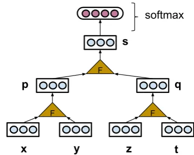
Figure 1: A recursive model (such as RNN and RLSTM) employ a composition function F in a bottom-up manner to compute a vector represen-tation for each internal node in a tree. If the model is used for classification on the sentence level, a softmax layer is put on the top of the root node to compute a distribution over all possible classes.

ferent tree depths, in which the key nodes which contain decisive information in a parse tree must be identified. Using available annotated corpora such as the Stanford Sentiment Treebank (Socher et al., 2013b) and the Penn Treebank is thus inap-propriate, as they are too small for this purpose (10k, 40k trees, respectively, compared to 240k trees in our experiments), and key nodes are not marked. Our solution is an artificial task where sentences and parse trees can be randomly gener-ated under any arbitrary constraints on tree depth and key node’s position.

2 Background

Both the RNN and the RLSTM model are in-stances of a general framework which takes a sen-tence, syntactic tree, and vector representations for the words in the sentence as input, and applies a composition function to recursively compute vec-tor representations for all the phrases in the tree and the complete sentence. Technically speaking, given a productionp→x y, andx,y∈Rn

repre-sentingx, y, we computep∈Rn_forpby

p=F(x,y)

whereF is a composition function (Figure 1). In the RNN,Fis a one-layer feed-forward neu-ral network:

p=f(W1x+W2y+b)

b∈R is a bias vector.fis an activation function. In the RLSTM, a node pis represented by the vector[p;cp]resulting from concatenating a

vec-tor representing the phrase that the node covers and a memory vector. F could be any LSTM that can compute two such concatenation vectors, such as Structure-LSTM (Zhu et al., 2015), Tree-LSTM (Tai et al., 2015), and Tree-LSTM-RNN (Le and Zuidema, 2015). In the current paper, we use the implementation1_{of Le and Zuidema (2015) where} an LSTM (for binary trees) has two input gates

i1, i2, two forget gates f1, f2, an output gate o, and a memory cell c. The vector representation and memory vector for node p are computed as follows:

i1 =σ Wi1x+Wi2y+Wci1cx+Wci2cy+bi

i2 =σ Wi1y+Wi2x+Wci1cy+Wci2cx+bi

f1 =σ Wf1x+Wf2y+Wcf1cx+Wcf2cy+bf

f2 =σ Wf1y+Wf2x+Wcf1cy+Wcf2cx+bf

cp =f1cx+f2cy+

g Wc1xi1+Wc2yi2+bc

o=σ Wo1x+Wo2y+Wcoc+bo

p=og(cp)

whereuandcu are the output and the state of the

memory cell at node u; i1, i2, f1, f2, o are the activations of the corresponding gates; W’s and b’s are weight matrices and bias vectors; andgis an activation function.

3 Experiments

We now examine how the two problems, the van-ishing gradient problem and the problem of how to capture long range dependencies, affect the RLSTM model and the RNN model. To do so, we propose the following artificial task, which re-quires a model to distinguish useful signals from noise. We define:

• a sentence is a sequence of tokens which are integer numbers in the range[0,10000]; • a sentence contains one and only onekeyword

token which is an integer number smaller than 1000;

• a sentence is labeled with the integer result-ing from dividresult-ing the keyword by 100. For

6

0

0

0

2 7 5 7 0

7 7 5 9

0

0

0

6 0 9 5 0

6 0 7

0

0

0

5 8 4 6 0

5 8 4 5

0

0

0

5 9 8 2 0

4 0 1 5

0

0

5 4 8 4 0

0

1 8 9 3 0

4 5 7 1

0

0

7 4 5 0

0

0

0

4 5 8 2 0

4 9 9 3 0

2 5 0 2

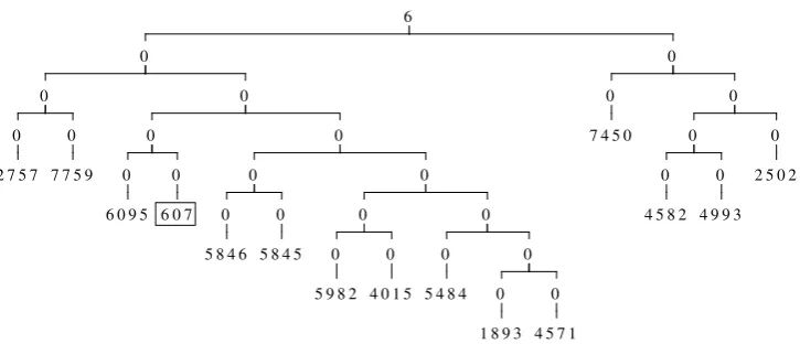
Figure 2: Example binary tree for the artificial task. The number enclosed in the box is thekeyword of the sentence.

instance, if the keyword is 607, the label is 6. In this way, there are 10 classes, ranging from 0 to 9.

The task is to predict the class of a sentence, given its binary parse tree (Figure 2). Because the label of a sentence is determined solely by the keyword, the two models need to identify the keyword in the parse tree and allow only the information from the leaf node of the keyword to affect the root node. It is worth noting that this task resembles sentiment analysis with simple cases in which the sentiment of a whole sentence is determined by one key-word (e.g. “I like the movie”). Simulating com-plex cases involving negation, composition, etc. is straightforward and for future work. But here we believe that the current task is adequate to answer our two questions raised in Section 1.

The two models, RLSTM and RNN, were im-plemented with the dimension of vector represen-tations and vector memories 50. Following Socher et al. (2013b), we used tanh as the activation function, and initialized word vectors by randomly sampling each value from a uniform distribution

U(−0.0001,0.0001). We trained the two models using the AdaGrad method (Duchi et al., 2011) with a learning rate of 0.05 and a mini-batch size of 20 for the RNN and of 5 for the RLSTM. De-velopment sets were employed for early stopping (training is halted when the accuracy on the de-velopment set is not improved after 5 consecutive epochs). It is worth noting that we also tried other values for the hyper-parameters but did not gain significantly better results on development sets.

3.1 Experiment 1

We randomly generated 10 datasets. To generate a sentence of lengthl, we shuffle a list of randomly chosenl−1non-keywords and one keyword. The

i-th dataset contains 12k sentences of lengths from

10i−9tokens to10itokens, and is split into train, dev, test sets with sizes of 10k, 1k, 1k sentences. We parsed each sentence by randomly generating a binary tree whose number of leaf nodes equals to the sentence length.

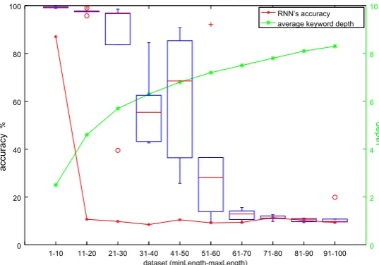
The test accuracies of the two models on the 10 datasets are shown in Figure 3; For each dataset we run each model 5 times and reported the high-est accuracy for the RNN model, and the distribu-tion of accuracies (via boxplot) for the RLSTM model. We can see that the RNN model per-forms reasonably well on very short sentences (less than 11 tokens). However, when the sentence length exceeds 10, the RNN’s performance drops so quickly that the difference between it and the random guess’ performance (10%) is negligible. Trying different learning rates, mini-batch sizes, and values forn(the dimension of vectors) did not give significant differences. On the other hand, the RLSTM model achieves more than 90% ac-curacy on sentences shorter than 31 tokens. Its performance drops when the sentence length in-creases, but is still substantially better than the ran-dom guess when the sentence length does not ex-ceed 70. When the sentence length exex-ceeds 70, both the RLSTM and RNN perform similarly.

3.2 Experiment 2

ex-1-10 11-20 21-30 31-40 41-50 51-60 61-70 71-80 81-90 91-100 0 2 4 6 8

datasetu(minLength-maxLength) 0

20 40 60 80

w

accuracy

depth

Figure 3: Test accuracies of the RNN (red solid curve, the best among 5 runs) and the RLSTM (boxplots) on datasets of different sentence lengths.

periment, we kept the tree size fixed and vary the keyword depth. We generated a pool of sentences of lengths from 21 to 30 tokens and parsed them by randomly generating binary trees. We then created 10 datasets each of which has 12k trees (10k for training, 1k for development, and 1k for testing). Thei-th dataset consists of only trees in which dis-tances from keywords to roots are i ori+ 1(to stop the networks from exploiting keyword depths directly).

Figure 4 shows test accuracies of the two mod-els on those 10 datasets. Similarly in Experiment 1, for each dataset we run each model 5 times and reported the highest accuracy for the RNN model, and the distribution of accuracies for the RLSTM model. As we can see, the RNN model achieves very high accuracies when the keyword depth does not exceed 3. Its performance then drops rapidly and gets close to the performance of the random guess. This is evidence that the RNN model has difficulty capturing long range de-pendencies. By contrast, the RLSTM model per-forms at above 90% accuracy until the depth of the keyword reaches 8. It has difficulty dealing with larger depths, but the performance is always better than the random guess.

3.3 Experiment 3

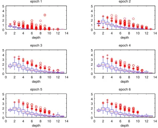
We now examine whether the two models can en-counter the vanishing gradient problem. To do so, we looked at the the back-propagation phase of each model in Experiment 1 on the third dataset (the one containing sentences of lengths from 21 to 30 tokens). For each tree, we calculated the

ra-tio

k_∂xkeyword∂J k k ∂J

∂xrootk

where the numerator is the norm of the error vector at the keyword node and the denominator is the norm of the error vector at the root node. This ratio gives us an intuition how the error signals develop when propagating backward to leaf nodes: if the ratio1, the vanishing gradient problem occurs; else if the ratio 1, we observe the exploding gradient problem.

1-2 2-3 3-4 4-5 5-6 6-7 7-8 8-9 9-10 10-11 0

20 40 60 80 100

dataset (minDepth-maxDepth)

%

accuracy

Figure 4: Test accuracies of the RNN (red solid curve, the best among 5 runs) and the RLSTM (boxplots) on datasets of different keyword depths.

0 2 4 6 8 10 12 14

0 1 2 3 4 5

depth epoch 1

0 2 4 6 8 10 12 14

0 1 2 3 4 5

depth epoch 2

0 2 4 6 8 10 12 14

0 1 2 3 4 5

depth epoch 3

0 2 4 6 8 10 12 14

0 1 2 3 4 5

depth epoch 4

0 2 4 6 8 10 12 14

0 1 2 3 4 5

depth epoch 5

0 2 4 6 8 10 12 14

0 1 2 3 4 5

depth epoch 6

Figure 5: Ratios of norms of error vectors at keyword nodes to norms of error vectors at root nodes w.r.t. the keyword node depth in each epoch of training the RNN. Gradients gradually vanish with greater depth.

to the keyword node. Comparing the two models by aligning Figure 5 with Figure 6, and Figure 7a with Figure 7b, we can see that the RLSTM model is more capable of transmitting error signals to leaf nodes.

It is worth noting that we do see the vanish-ing gradient problem happenvanish-ing when trainvanish-ing the RNN model in Figure 5; but Figure 7a suggests that the problem can become less serious after a

0 2 4 6 8 10 12 14 0

1 2 3 4

depth 0 2 4 6 8 10 12 14

0 1 2 3 4

depth

0 2 4 6 8 10 12 14

0 1 2 3 4 5

depth epoch 3

0 2 4 6 8 10 12 14

0 1 2 3 4 5

depth epoch 4

0 2 4 6 8 10 12 14

0 1 2 3 4 5

depth epoch 5

0 2 4 6 8 10 12 14

0 1 2 3 4 5

depth epoch 6

Figure 6: Ratios of norms of error vectors at keyword nodes (at different depths) to norms of error vectors at root nodes, in the RLSTM. Many gradients explode in epoch 2, but stabilize later. Gradients do not vanish, even at depth 12 and 13.

and capturing long term dependencies when train-ing traditional recurrent networks.

4 Conclusion

Because long range dependencies and vanishing gradients are serious challenges in deep learning, evaluating how well a model overcome these chal-lenges is necessary. In this current paper, we focus on two recursive models, RNN and RLSTM. Due to lack of natural data, we proposed a novel arti-ficial task where the label of a sentence is solely determined by a key word it contains. The exper-imental results show that the RLSTM is superior to the RNN. This is in parallel with general con-clusions about the power of the LSTM architec-ture compared to traditional Recurrent neural net-works.

Although our proposed task is simple, it is suf-ficient for testing recursive models since solving the task requires models to be capable of captur-ing long range dependencies and propagatcaptur-ing er-rors to leaf nodes far from the root. It is, moreover, straightforward to extend the task such that more complex cases can be taken into account. For in-stance, for compositionality, a sentence can con-tain more than one keywords and the sentence la-bel is determined by some kind of interaction

be-tween those keywords (such as addition).

References

Yoshua Bengio, Patrice Simard, and Paolo Frasconi. 1994. Learning long-term dependencies with

gra-dient descent is difficult. Neural Networks, IEEE

Transactions on, 5(2):157–166.

John Duchi, Elad Hazan, and Yoram Singer. 2011. Adaptive subgradient methods for online learning

and stochastic optimization. The Journal of

Ma-chine Learning Research, pages 2121–2159. Felix A Gers and J¨urgen Schmidhuber. 2001. Lstm

recurrent networks learn simple context-free and

context-sensitive languages. Neural Networks,

IEEE Transactions on, 12(6):1333–1340.

Sepp Hochreiter and J¨urgen Schmidhuber. 1997.

Long short-term memory. Neural computation,

9(8):1735–1780.

Phong Le and Willem Zuidema. 2015. Compositional distributional semantics with long short term

mem-ory. InProceedings of the Joint Conference on

Lex-ical and Computational Semantics (*SEM). Associ-ation for ComputAssoci-ational Linguistics.

Shujie Liu, Nan Yang, Mu Li, and Ming Zhou. 2014. A recursive recurrent neural network for statistical

machine translation. InProceedings of the 52nd

0 2 4 6 8 10 12 0

0.5 1 1.5 2 2.5 3

epoch

(a) RNN

0 2 4 6 8 10 120

20 40 60 80 100

epoch

%

0 0.5 1 1.5 2 2.5 3

accuracy

accuracy

(b) RLSTM (with development accuracies)

Figure 7: Ratios at depth 10 in each epoch of training the RNN (a) and the RLSTM (b).

Linguistics (Volume 1: Long Papers), pages 1491– 1500, Baltimore, Maryland, June. Association for Computational Linguistics.

Minh-Thang Luong, Richard Socher, and Christo-pher D Manning. 2013. Better word representa-tions with recursive neural networks for morphol-ogy. CoNLL-2013, 104.

Richard Socher, Christopher D. Manning, and An-drew Y. Ng. 2010. Learning continuous phrase representations and syntactic parsing with recursive

neural networks. InProceedings of the NIPS-2010

Deep Learning and Unsupervised Feature Learning Workshop.

Richard Socher, John Bauer, Christopher D Manning, and Andrew Y Ng. 2013a. Parsing with

compo-sitional vector grammars. In Proceedings of the

51st Annual Meeting of the Association for Compu-tational Linguistics, pages 455–465.

Richard Socher, Alex Perelygin, Jean Y Wu, Jason Chuang, Christopher D Manning, Andrew Y Ng, and Christopher Potts. 2013b. Recursive deep mod-els for semantic compositionality over a sentiment

treebank. InProceedings EMNLP.

Kai Sheng Tai, Richard Socher, and Christopher D. Manning. 2015. Improved semantic representa-tions from tree-structured long short-term memory

networks. InProceedings of the 53rd Annual

Meet-ing of the Association for Computational LMeet-inguistics and the 7th International Joint Conference on Natu-ral Language Processing (Volume 1: Long Papers), pages 1556–1566, Beijing, China, July. Association for Computational Linguistics.

Xiaodan Zhu, Parinaz Sobhani, and Hongyu Guo.

2015. Long short-term memory over recursive

structures. InProceedings of International