Proceedings of the 12th International Workshop on Semantic Evaluation (SemEval-2018), pages 732–740
SemEval-2018 Task 10: Capturing Discriminative Attributes
Alicia Krebs
Textkernel krebs@ textkernel.nl
Alessandro Lenci
University of Pisa alessandro.lenci@
unipi.it
Denis Paperno
Loria (UMR 7503), CNRS denis.paperno@
loria.fr
Abstract
This paper describes the SemEval 2018 Task 10 on Capturing Discriminative Attributes. Participants were asked to identify whether an attribute could help discriminate between two concepts. For example, a successful system should determine thaturineis a discriminating feature in the word pairkidney,bone. The aim of the task is to better evaluate the capabili-ties of state of the art semantic models, beyond pure semantic similarity. The task attracted submissions from 21 teams, and the best sys-tem achieved a 0.75 F1 score.
1 Introduction
State of the art semantic models do an excellent job at detecting semantic similarity, a traditional semantic task; for example, they can tell us that cappuccino, espresso and americano are similar to each other. It is obvious, however, that no model can claim to capture semantic competence if it does not, in addition to similarity, predict seman-tic differences between words. If one can tell that americano is similar to cappuccino and espresso but cannot tell the difference between them, one only has a very approximate idea of the meaning of these words. As a step beyond similarity, one should at the very least recognize that americano is bigger than espresso, and that capuccino contains milk foam. In this spirit, we present Semeval 2018 Task 10 (Capturing Discriminative Attributes) as a new challenge for lexical semantic models.
1.1 Task description
A semantic model that has only been evaluated on similarity detection may very well fail to be of practical use for specific applications. For ex-ample, word sense disambiguation could benefit greatly from representations that can model com-plex semantic relations. This means that the eval-uation of word representation models should not
only be centered on semantic similarity and relat-edness, and should include different, complemen-tary tasks. To fill this gap, we proposed a novel task of semantic difference detection as Task 10 of the SemEval 2018 workshop. The goal of the sys-tems in this case was to predict whether a word is a discriminative attribute between two other words. For example, given the wordsappleandbanana, is the wordreda discriminative attribute?
Semantic difference is a ternary relation be-tween two concepts (apple, banana) and a dis-criminative attribute (red) that characterizes the first concept but not the other. By its nature, se-mantic difference detection is a binary classifica-tion task: given a tripleapple,banana,red, the task is to determine whether it exemplifies a semantic difference or not.
In practice, when preparing the task, we started out with defining potential discriminative attributes as semantic features in the sense of (McRae et al.,2005): properties that people tend to think are important for a given concept. McRae et al.’s features are expressed as phrases, but these phrases can usually be reconstructed from a single word (e.g.redas a feature ofapplestands for the phraseis red,carpentryas a feature ofhammercan be used as a shorthand ofused for carpentry, etc.) Given this general reconstructability, we have for simplicity used single words rather than phrases to represent features. The same solution was also adopted in the feature norming studies by (Vinson and Vigliocco,2008) and (Lenci et al.,2013).
Following McRae et al., we did not define dis-criminative features in purely logical but rather in psychological terms. Accordingly, features are prototypical properties that subjects tend to asso-ciate to a certain concept. For example, not all ap-ples are red and some bananas are, butredtends to be judged as an important feature of apples and not of bananas. We therefore fully trust human
tators in deciding what counts as a distinguishing attribute and what does not.
1.2 Motivation
Exploring semantic differences between words can allow us to grasp subtle aspects of meaning: while it is relatively easy to train a model to rec-ognize thatappleandbananaare somewhat simi-lar, it is less straightforward to learn that, contrary to an apple, a typical banana is not red. This task is therefore more challenging than, and comple-mentary to, the traditional similarity task, and we expect it to contribute to the progress in computa-tional modeling of meaning.
While semantic similarity and relatedness mea-sures have been used extensively to evaluate se-mantic representations, they may not be sufficient as a method for evaluating lexical semantic mod-els (Faruqui et al.,2016;Batchkarov et al.,2016). Firstly, it has been noted that the relevant notions of similarity and relatedness can vary depending on the linguistic context, on the downstream ap-plication, etc. The difference task resolves this concern by effectively providing a context. In our example, comparison with bananas determines the relevance of the redness attribute for apples, which, out of context, might not necessarily be a salient attribute of apples.
Existing similarity and relatedness datasets have also been criticized for low inter-annotator agreement. The semantic difference detection task alleviates this issue, too. Binary choice is easier for human annotators than rating on a continuous scale, and produces more consistent patterns of an-swers. In our pilot study, the agreement between annotators was over 0.80. To further ensure the quality of our data, we discarded any items that caused disagreement.
1.3 Expected impact
The semantic difference task can enable further progress in the field of word representation learn-ing. Indeed, state of art models have reached ceil-ing performance in the tasks of semantic similar-ity and relatedness (in part because the ceiling, as determined by the agreement of human subjects, is relatively low). Another commonly employed task, analogy, has its own issues (Linzen, 2016) and effectivey boils down to similarity optimiza-tion (Levy and Goldberg, 2014). A new general evaluation task for lexical semantics is long due,
and we hope that the semantic difference task is capable of filling this gap.
In the future, solving the discriminative at-tributes task could help in a range of applica-tions, from conversational agents (choosing lex-ical items with contextually relevant differential features can help create more pragmatically appro-priate, human-like dialogues), to coreference res-olution (differentiating features of concepts men-tioned or alluded to in text could help in reference disambiguation), to machine translation and text generation, where explicitly taking into account semantic differences between competing transla-tion variants can improve the quality of the output.
2 Data and resources
2.1 Overview
One can express semantic differences between concepts by referring to attributes of those con-cepts. A difference can usually be expressed as presence or absence of a specific attribute. For in-stance, one of the differences between anarwhal
and adolphinis the presence of a tusk.
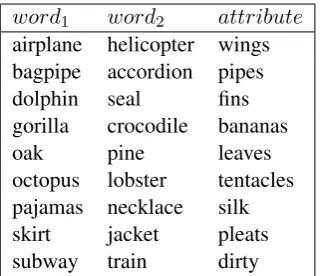
The task dataset includes 5062 manually veri-fied triples of the form<word1,word2,attribute>.
The set is built in such a way that the attribute in each positive example characterizes the first word of the triple. For example, in Table 1,
wings is an attribute ofairplane. The word pair
[airplane,helicopter]is included in the order[helicopter,airplane]ifhelicopter
has a feature that airplane does not have. We thereby assume, in contrast to the standard for-malization of similarity, that semantic difference is not symmetric: the triple apple,banana,red is a semantic difference butbanana,apple,redis not sinceredis not an attribute of bananas.1
We supplemented positive data (as described above) with negative examples. Two types of negative examples were added: examples where the attribute is shared betweenword1 andword2
(both concepts have the attribute in question), and examples where the attribute is neither an attribute of word1 nor word2 (both concepts lack the
at-tribute). For that last type of attributes, since their 1This is a somewhat arbitrary choice. One could
word1 word2 attribute
airplane helicopter wings bagpipe accordion pipes
dolphin seal fins
gorilla crocodile bananas
oak pine leaves
octopus lobster tentacles pajamas necklace silk
skirt jacket pleats
[image:3.595.102.263.61.199.2]subway train dirty
Table 1: Sample data: Word pairs and their distinguish-ing features (positive examples)
number is potentially huge, the examples were se-lected randomly so that the number of negative ex-amples matches the number of positive exex-amples. Presence of both positive and negative examples makes it possible to train a binary classifier that, for a given triple, predicts whether the attribute is a difference betweenword1 andword2.
word1 word2 attribute
tractor scooter wheels
crow owl black
squirrel leopard fur
pillow jacket white
dresser cupboard large spider elephant legs
gloves pants wool
gorilla panther long scarf slippers colours
lion zebra large
Table 2: Sample data: Word pairs and non-distinguishing features (negative examples)
Approximately half of the manually checked triples was given to participants as a validation set for parameter tuning of their systems, the rest was used for testing (cf. Section2.4 for detailed statistics about the dataset composition). A larger training set of almost 18K examples (automati-cally constructed by the procedure described be-low, without manual filtering) was provided for training parameter-rich systems.
2.2 Data collection and annotation
When creating the dataset, we started from the ap-proach thatLazaridou et al.(2016) used for visual discriminating attribute identification, followed by manual filtering for the test and validation data. Dataset creation consisted of three phases:
1. Semi-automatically created triples (section 2.2.1)
2. Manually created triples (section2.2.2)
3. Automatically created triples (section2.2.3)
As an initial source of data, we used the fea-ture norms collected by McRae et al. (2005) and created a pilot dataset (Krebs and Paperno,2016). This set was then reverified and manually ex-tended to improve the quality and the variety of the data. Finally, a large number of triples were automatically generated for training purposes.
2.2.1 Triples from Mcrae norms
The first part of the dataset was created semi-automatically by identifying discriminative at-tributes of the concepts in the McRae norms, which consist of a list of features for 541 concepts (living and non-living entities), collected by ask-ing 725 participants to produce features for each concept. Production frequencies of these attributes indicate how salient they are. Concepts that have different meanings had been disambiguated be-fore being shown to participants. For example, there are two entries for bow, bow (weapon)
andbow (ribbon).
Because our task is not intended to test word sense models, we did not differentiate between en-tries that have multiple senses and ignored the dis-ambiguating phrase. In our dataset, the concept
bowhas the attributes of both the weapon and the ribbon. This is not problematic because we do not refer to more than one attribute at a time, so senses of a word do not mix.2The McRae dataset uses the
brain region taxonomy (Cree and McRae, 2003) to classify attributes into different types, such as
function, sound ortaxonomic. For the construc-tion of our dataset, we decided to only work with visual attributes, which exist for all concrete con-cepts, while attributes such as sound ortasteare only relevant for some classes of concepts.
Any one word concept that has at least one vi-sual attribute was considered a candidate. Each 2An anonymous reviewer points out that the presence or
absence of a feature inw1can be influenced by the context
ofw2: e.g.tailcould be considered a distinguishing feature
[image:3.595.105.257.355.506.2]candidate concept was paired with another candi-date concept from the list of its 100 closest neigh-bours in a PPMI-based distributional vector space (using the best settings fromBaroni et al.(2014)). The motivation for this step is that finding non-trivial semantic differences only makes sense in the context of related words; detecting the differ-ence between two unrelated concepts, such as a narwhal and a tractor, is rather trivial and would not constitute a very interesting task.
For each word pair, if there was an attribute in McRae feature norms that the first word has but the second doesn’t, the word pair – attribute triple was added to the list of candidate positive examples. For simplicity, multi-word attributes were processed so that only the last word is taken into account (e.g.has wingsbecomeswings). At this point, we had 512 unique concepts, 1645 unique attributes, 6355 unique word pairs, and 41723 triples (word pair-concept combinations). A random sample of triples was selected for man-ual annotation.
For candidate positive examples, two annotators agreed to keep 45.2% of items, agreed to discard 33% of items, and disagreed on 21.8% of items. A total of 54.8% of candidate positive examples were discarded. Among the negative examples, 12.5% of items were discarded. Annotators agreed to keep 87.5% of items, agreed to discard 0.8% of items, and disagreed on 11.6% of items. The ex-amples that both annotators agreed to discard from the positive examples were added to the negative examples. Finally, the third author manually fil-tered the data removing dubious examples.
2.2.2 Manual triples
In the second phase, we extended the dataset by adding new concepts and attributes. Our intention was to make the dataset more diverse and more representative of the noun lexicon by including words and features that are not part of the McRae feature norms (e.g., human nouns such as doctor
orstudent).
To select new nouns, we used SimLex-999 (Hill et al., 2015), one of the largest and most popu-lar datasets for semantic simipopu-larity. We extracted from SimLex all the nouns with a concreteness rating above the median, and identified 204 can-didate items that were not included in the McRae Norms. Each selected noun was paired with candi-date concepts from the list of its 20 closest neigh-bours in the distributional vector space. We then
filtered the neighbors by frequency, keeping the neighbors that belong to the frequency range of the original McRae and SimLex vocabulary. We also made sure at this step that candidate word pairs be-long to the same WordNet supersense. This latter constraint was added because distributional mod-els often return neighbors that are only loosely re-lated to the target, while finding non-trivial seman-tic differences makes sense only for words that are taxonomically similar. We also discarded gram-matical number pairs like seed/seeds and hyper-nym/hyponym pairs likedoctor/surgeon, since by definition there is no feature that a hypernym has but its hyponym does not have.
Each of the three task organizers was given a third of the resulting 1851 candidate noun pairs to annotate, generating discriminative and non-discriminative attributes for each pair. The sug-gested triples were then manually filtered by the other two authors.
2.2.3 Random triples
Finally, to further ensure the diversity of exam-ples and to alleviate any biases unintentionally introduced in the annotation pipeline, we gener-ated 500 additional triples by randomly match-ing words and features produced at earlier stages. Each of the three authors annotated these ran-dom triples, which contained mainly negative ( mo-torbike,rifle,liquor) and some positive examples (e.g.maid,evening,help). Again, only those exam-ples for which a full consensus of the three authors existed were kept.
2.3 Training, test and validation partitions
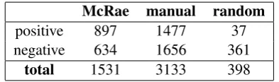
The manually validated dataset of semantic dif-ferences consists of examples from three sources described above: combinations of nouns with McRae features, triples with manually suggested attributes, and random triples. All of these exam-ples have been verified by the three authors and were then randomly split into a validation partition and a test partition, making sure that no feature oc-curs in both.
McRae manual random
positive 897 1477 37
negative 634 1656 361
[image:4.595.318.515.676.734.2]total 1531 3133 398
To enable development of systems that require more training data, we also created a distinct, big-ger training set that was not manually curated. The training set was derived from McRae feature norms using automatically matched examples as described in 2.1.1, but without manual validation. We have to note that this training partition is very noisy, its main advantage being its size. In fact, the best performing system in our task was trained directly on validation data.
We further filtered the training set to minimize lexical overlap between partitions, making sure that no attribute present in the test set or the vali-dation set is also present in the training set. For example, if the attribute “red” appears in some triple in the test partition, you will not find it any-where in the training set. This was done to ensure that models cannot rely on attribute memorization from training data but are forced to transfer lexical knowledge from other sources.
2.4 Dataset composition
The final dataset consists of 22884 items, divided into:
1. A training set of 17782 examples with 515 distinct concepts and 1292 distinct features.
2. A validation set of 2722 examples with 1283 concepts and 576 distinct features.
3. A test set of 2340 triples with 1272 distinct concepts and 577 distinct features.
The proportion of positive and negative examples is reported in Table2.4.
training validation testing
positive 6591 1364 1047
negative 11191 1358 1293
total 17782 2722 2340
Table 4: Total size of the final dataset.
All data used in this task can be accessed from the competition’s github repository.3
3 Evaluation
3.1 Metrics
The submitted systems were evaluated on F1 mea-sure, as is standard in binary classification tasks.
3https://github.com/dpaperno/DiscriminAtt/
The evaluation script can be found in the compe-tition’s github repository. The competition results can be seen at the corresponding Codalab page.4
Participants were allowed to make up to 2 submis-sions, resulting in 47 total submissions from 28 different teams (but only 21 teams submitted pa-pers). Only the better of the two submissions of each team is included in final results.
3.2 Baselines
Since our task is formalized as binary classifica-tion, the random baseline has 0.50 accuracy. As our test set is not perfectly balanced, a most fre-quent class baseline would get 0.517 F1.
We also computed an unsupervised distribu-tional vector cosine baseline based on the idea that a discriminative attribute is close to the word it characterizes and further away from the other member of the pair. In the cosine method, each item is classified as a semantic difference if the co-sine similarity ofword1and the attribute is greater
than the cosine similarity of word2 and the
at-tribute. To compute the cosine baseline, we used a PPMI-based vector space with the best settings fromBaroni et al.(2014).
The cosine baseline correctly classifies 0.691 of positive items and 0.539 of negative items in the test data, which corresponds to an average F1 mea-sure of 0.607.
3.3 Human upper bound
correct incorrect
positive 724 323
[image:6.595.106.256.62.105.2]negative 697 596
Table 5: Number of correct and incorrect classifications for the test set using the cosine baseline.
Rank Team Score
1 SUNNYNLP 0.75
2 Luminoso 0.74
3 BomJi 0.73
3 NTU NLP 0.73
4 UWB 0.72
5 ELiRF-UPV 0.69
5 Meaning Space 0.69
5 Wolves 0.69
6 Discriminator 0.67
6 ECNU 0.67
5 AmritaNLP 0.66
6 GHH 0.65
7 ALB 0.63
7 CitiusNLP 0.63
7 THU NGN 0.63
8 UNBNLP 0.61
9 UNAM 0.60
10 UMD 0.60
11 ABDN 0.52
12 Igevorse 0.51
13 bicici 0.47
ceiling human 0.90
[image:6.595.345.489.62.105.2]baselines (strong) cosine 0.607 (weak) random 0.517
Table 6: Codalab competition results, compared to baselines and the human-based performance ceiling.
System type Count Average F1 Best F1
NN 4 0.66 0.73
Rule-based 7 0.63 0.69
SVM / SVC 6 0.68 0.75
XGB 2 0.70 0.73
Table 7: Average and best F1 score per system type.
4 Systems Overview
Table6shows the best performing system submit-ted by each participating team which submitsubmit-ted descriptions of their systems.
Many participants created custom rules to tackle the task, using for example cosine
similar-4https://competitions.codalab.org/competitions/17326
Resource type Average F1
WE + KB 0.678
WE 0.638
Table 8: Average F1 score per resource type (KB = Knowledge Base, WE = Word Embeddings).
ity or co-occurrence frequency thresholds (Mean-ing Space,Sommerauer et al.; ELiRF-UPV, Gon-zlez et al.; CitiusNLP Gamallo; UNAM Arroyo-Fernndez et al.; Discriminator, Kulmizev et al.; UNBNLP, King et al.; ABDN, Mao et al.; Igevorse,Grishin).
Some of the most successful systems employed traditional machine learning algorithms such as SVMs (SUNNYNLP, Lai et al.; ALB, Dumitru et al.; Wolves, Taslimipoor et al.; ECNU, Zhou et al.; UMD, Zhang and Carpuat), SVC (Lumi-noso,Speer and Lowry-Duda) and Maximum En-tropy Classifiers (UWB,Brychcn et al.).
Other teams chose to build their systems us-ing deep learnus-ing systems such as neural networks (GHH, Attia et al.; Shiue et al.), CNNs (THU NGN,Wu et al.; AmritaNLP,Vinayan et al.) and XGB classifiers (BomJi, Santus et al.; ECNU, Zhou et al.).
Participants made use of a large number of re-sources. Such resources can be divided into word embeddings (e.g., Word2Vec, GloVe, fastText) and knowledge base type resources (e.g., Word-Net, ConceptWord-Net, Probase). Participants’ analyses of their results indicate that although using knowl-edge bases can yield high precision results, they cannot easily cover all cases. When employing pre-trained word embeddings, participants noted that out-of-vocabulary items become a challenge. But most importantly, a shortcoming of word em-beddings with regard to our task is their inability to distinguish between different types of semantic re-latedness. As noted by the GHH team (Attia et al.),
garlicis related towingsnot because garlic has the ability to fly but because garlic chicken wings are a popular dish choice; a shallow cooccurence-based model will fail to recognize that wings character-ize chicken but not garlic.
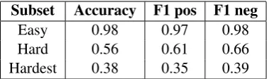
[image:6.595.93.270.132.495.2] [image:6.595.96.268.151.493.2] [image:6.595.72.293.541.612.2]Subset Accuracy F1 pos F1 neg
Easy 0.98 0.97 0.98
Hard 0.56 0.61 0.66
[image:7.595.87.277.62.118.2]Hardest 0.38 0.35 0.39
Table 9: Results of human annotation of the Easy, Hard and Hardest subsets of the test data.
5 Results analysis
We have carried out an in-depth exploration of the systems results in order to get a better insight on the relationship between their performance and the dataset structure and complexity. We ranked all the test triples by the number of systems that an-notated them correctly and we selected the 50 top triples that were scored correctly by the most sys-tems and the 50 top triples that were failed by most systems. We called these two subsets theEasyand theHarddata, respectively. Then, we focused on the results produced by the top 5 systems in Ta-ble 6, with an overall performance greater than 70%. Out of the 1340 triples that were failed by at least one of these top systems, we selected the 112 triples (8.3%) that were failed by all 5
sys-tems. We called this subset the Hardest data. These datasets were annotated by the same three expert annotators used to compute the human up-per bound (cf. Section 3.3). The accuracy and F1 of the aggregated human judgments (majority vote) with respect to the gold standard are reported in Table9.
The annotation results show an interesting cor-relation between the system and human perfor-mances. The “easy” triples for the systems are easy for humans too, and conversely the harder a triple is for a system the harder it is for humans. The lowest annotation accuracy is on the Hardest subset, less than40%. However, since this set con-tains the triples that were failed by all top systems, the human accuracy also proves that theres is still plenty of room for improvement even for the best performing models.
Table9shows that the F1 on the negative class is usually higher than the one on the positive class. This is again similar to systems behavior. In fact, 70% of the top 100 triples scored correctly by most systems are negative cases, while67%of the top 100 triples failed by most systems are positive cases. The 112 triples failed by all top file systems contain54%positive cases. This suggests that for systems and humans alike it is usually harder to
McRae manual random
label pos neg pos neg pos neg
Easy 1 9 20 7 13 0
Hard 8 2 12 26 0 2
Table 10: Example label and source distribution for the Easy and Hard subsets of the test data.
identify a discriminative attribute, rather than a non-discriminative one. Finally, out of the 1340 triples that were failed by at least one of the top 5 systems, 502 (37%) were failed by just one model. This shows that a great variance exists in the be-havior and in the weaknesses of these systems, de-spite their very close performance.
Types of attributes seem to vary in how difficult they are to differentiate in the context of our task. For example, attributes that stand in the whole-part relation with the word, as indoor,gate,handle, lean on the hard side (9 examples in the Hard sam-ple vs. 2 in the Easy one). Attributes that are adjectives, as in rods,wire,hard, also tend to be hard (25 examples in theHard sample vs. 13 in the Easyone), presumably because of the gradi-ent and context-dependgradi-ent meaning of adjectives; indeed, 9 of the 13 “easy” examples with adjec-tive attributes involve colours, which are relaadjec-tively context-independent (as opposed to 4 colour out of the 25 “hard” adjective examples).
[image:7.595.314.517.62.119.2]ac-tress, but not for artist. The former type of prob-lems prompt for a further revision of the gold stan-dard, while the latter type reveals the complexity of the notion of discriminative attribute and its dif-ficult applications in some cases, which will re-quire a deeper specification of annotation guide-lines.
6 Conclusion
Discriminative attribute detection is an intuitively simple and appealing yet challenging new task for lexical semantic systems. For the SemEval com-petition, we created a high quality dataset of se-mantic differences, with estimated ceiling perfor-mance of human annotators of 0.90. While the task is far from being solved, participating systems showed promising results, most of them beating the cosine baseline.
It is clear that learning to discriminate differen-tiating features is not trivial and requires training, both for human annotators and for computational systems; all of the top performing systems used machine learning techniques of some kind.
While different teams employed different lin-guistic resources, the results of the competition do not allow us to conclude that a particular re-source gives one’s system an edge. On the one hand, exploiting information from knowledge base resources like WordNet does improve the perfor-mance on average. On the other hand, traditional machine learning systems that entered our com-petition were much more likely to make use of knowledge bases. Therefore, combining neural approaches with knowledge bases may very well lead to improved performances.
As we mentioned above, ceiling performance has already been achieved in traditional tasks such as word similarity, causing a stagnation of lexical semantic modeling. As the best systems in our competition showed very promising results, we hope to see novel semantic models demonstrate their full potential on our task.
Acknowledgements
We thank Marco Baroni, Roberto Zamparelli, and three anonymous reviewers for their helpful com-ments. We thank Giulia Cappelli, Patrick Jeu-nieaux, and Marco Senaldi for their valued support in the data analysis. This work was supported by the CNRS PEPS I3A project ReSeRVe.
References
Ignacio Arroyo-Fernndez, Carlos-Francisco Mendez-Cruz, and Ivan Meza. 2018. Unam at semeval-2018 task 10: Unsupervised semantic discrimina-tive attribute identification in neural word embed-ding cones. InProceedings of the 12th international workshop on semantic evaluation (SemEval 2018).
Mohammed Attia, Younes Samih, Manaal Faruqui, and Wolfgang Maier. 2018. Ghh at semeval-2018 task 10: Discovering discriminative attributes in distri-butional semantics. InProceedings of the 12th inter-national workshop on semantic evaluation (SemEval 2018).
Marco Baroni, Georgiana Dinu, and Germ´an Kruszewski. 2014. Don’t count, predict! a systematic comparison of context-counting vs. context-predicting semantic vectors. In ACL (1), pages 238–247.
Miroslav Batchkarov, Thomas Kober, Jeremy Reffin, Julie Weeds, and David Weir. 2016. A critique of word similarity as a method for evaluating distri-butional semantic models. In First Workshop on Evaluating Vector Space Representations for NLP (RepEval 2016).
Tom Brychcn, Tom Hercig, Josef Steinberger, and Michal Konkol. 2018. Uwb at semeval-2018 task 10: Capturing discriminative attributes from word distributions. In Proceedings of the 12th interna-tional workshop on semantic evaluation (SemEval 2018).
George S Cree and Ken McRae. 2003. Analyzing the factors underlying the structure and computation of the meaning of chipmunk, cherry, chisel, cheese, and cello (and many other such concrete nouns). Journal of Experimental Psychology: General, 132(2):163.
Bogdan Dumitru, Alina Maria Ciobanu, and P. Dinu Liviu. 2018. Alb at semeval-2018 task 10: A system for capturing discriminative attributes. In Proceed-ings of the 12th international workshop on semantic evaluation (SemEval 2018).
Manaal Faruqui, Yulia Tsvetkov, Pushpendre Rastogi, and Chris Dyer. 2016. Problems with evaluation of word embeddings using word similarity tasks. In First Workshop on Evaluating Vector Space Repre-sentations for NLP (RepEval 2016).
Pablo Gamallo. 2018. Citiusnlp at semeval-2018 task 10: The use of transparent distributional models and salient contexts to discriminate word. In Proceed-ings of the 12th international workshop on semantic evaluation (SemEval 2018).
Maxim Grishin. 2018. Igevorse at semeval-2018 task 10: Exploring an impact of word embeddings con-catenation for capturing discriminative attributes. In Proceedings of the 12th international workshop on semantic evaluation (SemEval 2018).
Felix Hill, Roi Reichart, and Anna Korhonen. 2015. Simlex-999: Evaluating semantic models with (gen-uine) similarity estimation. Computational Linguis-tics, 41(4):665–695.
Milton King, Ali Hakimi Parizi, and Paul Cook. 2018. Unbnlp at semeval-2018 task 10: Evaluating unsu-pervised approaches to capturing discriminative at-tributes. In Proceedings of the 12th international workshop on semantic evaluation (SemEval 2018). Alicia Krebs and Denis Paperno. 2016. Capturing
dis-criminative attributes in a distributional space: Task proposal. In Proceedings of RepEval 2016: The First Workshop on Evaluating Vector Space Repre-sentations for NLP.
Artur Kulmizev, Mostafa Abdou, Vinit Ravishankar, and Malvina Nissim. 2018. Discriminator at semeval-2018 task ten: Zero-shot discrimination. In Proceedings of the 12th international workshop on semantic evaluation (SemEval 2018).
Sunny Lai, Kwong Sak Leung, and Yee Leung. 2018. Sunnynlp at semeval-2018 task 10: A support-vector-machine-based method for detecting seman-tic difference using taxonomy and word embedding features. In Proceedings of the 12th international workshop on semantic evaluation (SemEval 2018). Angeliki Lazaridou, Nghia The Pham, and Marco
Ba-roni. 2016. The red one!: On learning to refer to things based on their discriminative properties. arXiv preprint arXiv:1603.02618.
Alessandro Lenci, Marco Baroni, Giulia Cazzolli, and Giovanna Marotta. 2013. BLIND: a set of semantic feature norms from the congenitally blind. Behavior Research Methods, 45(4):1218–1233.
Omer Levy and Yoav Goldberg. 2014. Linguistic reg-ularities in sparse and explicit word representations. InProceedings of the eighteenth conference on com-putational natural language learning, pages 171– 180.
Tal Linzen. 2016. Issues in evaluating seman-tic spaces using word analogies. arXiv preprint arXiv:1606.07736.
Rui Mao, Guanyi Chen, Ruizhe Li, and Chenghua Lin. 2018. Abdn at semeval-2018 task 10: Recognising discriminative attributes using context embeddings and wordnet. In Proceedings of the 12th interna-tional workshop on semantic evaluation (SemEval 2018).
Ken McRae, George S Cree, Mark S Seidenberg, and Chris McNorgan. 2005. Semantic feature produc-tion norms for a large set of living and nonliving things. Behavior research methods, 37(4):547–559.
Enrico Santus, Chris Biemann, and Emmanuele Cher-soni. 2018. Bomji at semeval-2018 task 10: Com-bining vector-, pattern- and graph-based information to identify discriminative attributes. InProceedings of the 12th international workshop on semantic eval-uation (SemEval 2018).
Yow-Ting Shiue, Hen-Hsen Huang, and Hsin-Hsi Chen. 2018. Ntu nlp lab system at semeval-2018 task 10: Verifying semantic differences by integrat-ing distributional information and expert knowledge. In Proceedings of the 12th international workshop on semantic evaluation (SemEval 2018).
Pia Sommerauer, Antske Fokkens, and Piek Vossen. 2018. Meaning space at semeval-2018 task 10: Combining explicitly encoded knowledge with in-formation extracted from word embeddings. In Pro-ceedings of the 12th international workshop on se-mantic evaluation (SemEval 2018).
Robert Speer and Joanna Lowry-Duda. 2018. Lumi-noso at semeval-2018 task 10: Distinguishing at-tributes using text corpora and relational knowledge. In Proceedings of the 12th international workshop on semantic evaluation (SemEval 2018).
Shiva Taslimipoor, Omid Rohanian, and Le An Ha. 2018. Wolves at semeval-2018 task 10: Semantic discrimination based on knowledge and association. In Proceedings of the 12th international workshop on semantic evaluation (SemEval 2018).
Vivek Vinayan, Anand Kumar, and K P Soman. 2018. Amritanlp@semeval-2018 task 10: Capturing dis-criminative attributes using convolution neural net-work over global vector representation. In Proceed-ings of the 12th international workshop on semantic evaluation (SemEval 2018).
David P Vinson and Gabriella Vigliocco. 2008. Se-mantic feature production norms for a large set of objects and events. Behavior Research Methods, 40(1):183–190.
Chuhan Wu, Fangzhao Wu, Sixing Wu, Zhigang Yuan, and Yongfeng Huang. 2018. Thu ngn at semeval-2018 task 10: Capturing discriminative attributes with mlp-cnn model. In Proceedings of the 12th international workshop on semantic evaluation (Se-mEval 2018).
Alexander Zhang and Marine Carpuat. 2018. Umd at semeval-2018 task 10: Can word embeddings cap-ture discriminative attributes? InProceedings of the 12th international workshop on semantic evaluation (SemEval 2018).