Dynamic Language Models for Streaming Text
Dani Yogatama∗ Chong Wang∗ Bryan R. Routledge† Noah A. Smith∗ Eric P. Xing∗ ∗School of Computer Science
†Tepper School of Business Carnegie Mellon University Pittsburgh, PA 15213, USA
∗{dyogatama,chongw,nasmith,epxing}@cs.cmu.edu, †[email protected]
Abstract
We present a probabilistic language model that captures temporal dynamics and conditions on arbitrarynon-linguisticcontext features. These context features serve as important indicators of language changes that are otherwise difficult to capture using text data by itself. We learn our model in an efficient online fashion that is scalable for large, streaming data. With five streaming datasets from two different genres— economics news articles and social media—we evaluate our model on the task of sequential language modeling. Our model consistently outperforms competing models.
1 Introduction
Language models are a key component in many NLP applications, such as machine translation and ex-ploratory corpus analysis. Language models are typi-cally assumed to be static—the word-given-context distributions do not change over time. Examples includen-gram models (Jelinek, 1997) and proba-bilistic topic models like latent Dirichlet allocation (Blei et al., 2003); we use the term “language model” to refer broadly to probabilistic models of text.
Recently, streaming datasets (e.g., social media) have attracted much interest in NLP. Since such data evolve rapidly based on events in the real world, as-suming a static language model becomes unrealistic. In general, more data is seen as better, but treating all past data equally runs the risk of distracting a model with irrelevant evidence. On the other hand, cau-tiously using only the most recent data risks overfit-ting to short-term trends and missing important time-insensitive effects (Blei and Lafferty, 2006; Wang et al., 2008). Therefore, in this paper, we take steps toward methods for capturing long-range temporal dynamics in language use.
Our model also exploits observable context vari-ables to capture temporal variation that is otherwise difficult to capture using only text. Specifically for the applications we consider, we use stock market data as exogenous evidence on which the language model depends. For example, when an important company’s price moves suddenly, the language model should be based not on the very recent history, but should be similar to the language model for a day when a similar change happened, since people are likely to say similar things (either about that com-pany, or about conditions relevant to the change). Non-linguistic contexts such as stock price changes provide useful auxiliary information that might indi-cate the similarity of language models across differ-ent timesteps.
We also turn to a fully online learning framework (Cesa-Bianchi and Lugosi, 2006) to deal with non-stationarity and dynamics in the data that necessitate adaptation of the model to data in real time. In on-line learning, streaming examples are processed only when they arrive. Online learning also eliminates the need to store large amounts of data in memory. Strictly speaking, online learning is distinct from
stochasticlearning, which for language models built on massive datasets has been explored by Hoffman et al. (2013) and Wang et al. (2011). Those tech-niques are still for static modeling. Language model-ing for streammodel-ing datasets in the context of machine translation was considered by Levenberg and Os-borne (2009) and Levenberg et al. (2010). Goyal et al. (2009) introduced a streaming algorithm for large scale language modeling by approximatingn -gram frequency counts. We propose a general online learning algorithm for language modeling that draws inspiration from regret minimization in sequential predictions (Cesa-Bianchi and Lugosi, 2006) and
line variational algorithms (Sato, 2001; Honkela and Valpola, 2003).
To our knowledge, our model is the first to bring together temporal dynamics, conditioning on non-linguistic context, and scalable online learning suit-able for streaming data and extensible to include topics andn-gram histories. The main idea of our model is independent of the choice of the base lan-guage model (e.g., unigrams, bigrams, topic models, etc.). In this paper, we focus on unigram and bi-gram language models in order to evaluate the basic idea on well understood models, and to show how it can be extended to higher-ordern-grams. We leave extensions to topic models for future work.
We propose a novel task to evaluate our proposed language model. The task is to predict economics-related text at a given time, taking into account the changes in stock prices up to the corresponding day. This can be seen an inverse of the setup considered by Lavrenko et al. (2000), where news is assumed to influence stock prices. We evaluate our model on economics news in various languages (English, German, and French), as well as Twitter data.
2 Background
In this section, we first discuss the background for sequential predictions then describe how to formulate online language modeling as sequential predictions.
2.1 Sequential Predictions
Letw1, w2, . . . , wT be a sequence of response
vari-ables, revealed one at a time. The goal is to design a good learner to predict the next response, given previous responses and additional evidence which we denote byxt∈RM (at timet). Throughout this
paper, we use the termfeaturesforx. Specifically, at each roundt, the learner receivesxtand makes a
pre-dictionwˆt, by choosing a parameter vectorαt∈RM.
In this paper, we refer toαasfeature coefficients. There has been an enormous amount of work on online learning for sequential predictions, much of it building on convex optimization. For a sequence of loss functions`1, `2, . . . , `T (parameterized byα),
an online learning algorithm is a strategy to minimize the regret, with respect to the best fixedα∗ in hind-sight.1 Regret guarantees assume a Lipschitz
con-1Formally, the regret is defined as Regret
T(α∗) =
dition on the loss function`that can be prohibitive for complex models. See Cesa-Bianchi and Lugosi (2006), Rakhlin (2009), Bubeck (2011), and Shalev-Shwartz (2012) for in-depth discussion and review.
There has also been work on online and stochastic learning for Bayesian models (Sato, 2001; Honkela and Valpola, 2003; Hoffman et al., 2013), based on variational inference. The goal is to approximate pos-terior distributions of latent variables when examples arrive one at a time.
In this paper, we will use both kinds of techniques to learn language models for streaming datasets.
2.2 Problem Formulation
Consider an online language modeling problem, in the spirit of sequential predictions. The task is to build a language model that accurately predicts the texts generated on day t, conditioned on observ-able features up to day t, x1:t. Every day, after
the model makes a prediction, the actual texts wt
are revealed and we suffer a loss. The loss is de-fined as the negative log likelihood of the model `t=−logp(wt |α,β1:t−1,x1:t−1,n1:t−1), where
αandβ1:T are the model parameters andnis a back-ground distribution (details are given in§3.2). We can then update the model and proceed to dayt+ 1. Notice the similarity to the sequential prediction de-scribed above. Importantly, this is a realistic setup for building evolving language models from large-scale streaming datasets.
3 Model 3.1 Notation
We index timesteps by t ∈ {1, . . . , T} and word types byv ∈ {1, . . . , V}, both are always given as subscripts. We denote vectors in boldface and use 1 : T as a shorthand for{1,2, . . . , T}. We assume words of the form{wt}Tt=1 forwt ∈RV, which is
the vector of word frequences at timetstept. Non-linguistic context features are{xt}Tt=1forxt∈RM.
The goal is to learn parametersαandβ1:T, which will be described in detail next.
3.2 Generative Story
The main idea of our model is illustrated by the fol-lowing generative story for the unigram language
PT
t=1`t(xt,αt, wt)−infα∗
PT
model. (We will discuss the extension to higher-order language models later.) A graphical representation of our proposed model is given in Figure 1.
1. Draw feature coefficientsα∼N(0, λI).2 Here αis a vector inRM, whereM is the
dimension-ality of the feature vector. 2. For each timestept:
(a) Observe non-linguistic context featuresxt.
(b) Drawβt∼
N
Pt−1
k=1δk
exp(α>f(xt,xk))
Pt−1
j=1δjexp(α>f(xt,xj))βk, ϕI
. Here, βt is a vector in RV, where V is the size of the word vocabulary, ϕ is the variance parameter and δk is a fixed
hyperparameter; we discuss them below. (c) For each word wt,v, draw wt,v ∼
Categorical exp(n1:t−1,v+βt,v)
P
j∈Vexp(n1:t−1,j+βt,j)
. In the last step, βt and n are mapped to the V -dimensional simplex, forming a distribution over words. n1:t−1 ∈ RV is a background (log)
distri-bution, inspired by a similar idea in Eisenstein et al. (2011). In this paper, we setn1:t−1,vto be the
log-frequency ofvup to timet−1. We can interpretβ as a time-dependent deviation from the background log-frequencies that incorporates world-context. This deviation comes in the form of a weighted average of earlier deviation vectors.
The intuition behind the model is that the probabil-ity of a word appearing at daytdepends on the back-ground log-frequencies, the deviation coefficients of the word at previous timestepsβ1:t−1, and the sim-ilarity of current conditions of the world (based on observable featuresx) to previous timesteps through f(xt,xk). That is, f is a function that takes d
-dimensional feature vectors at two timestepsxtand xkand returns a similarity vectorf(xt,xk)∈RM
(see§6.1.1 for an example off that we use in our experiments). The similarity is parameterized byα, and decays over time with rateδk. In this work, we
assume a fixed window sizec (i.e., we considerc most recent timesteps), so that δ1:t−c−1 = 0 and
δt−c:t−1 = 1. This allows up to cth order
depen-dencies.3 Settingδthis way allows us to bound the 2Feature coefficientsαcan be also drawn from other
distri-butions such asα∼Laplace(0, λ).
3In online Bayesian learning, it is known that forgetting
inaccurate estimates from earlier timesteps is important (Sato,
x
t
x
s
x
r
x
q
w
q
w
r
ws
wt
t
s
r
q
↵
N
rNq
N
sN
t [image:3.612.321.534.58.239.2]T
Figure 1: Graphical representation of the model. The subscript indices q, r, s are shorthands for the
previ-ous timestepst−3, t−2, t−1. Only four timesteps are shown here. There are arrows from previous βt−4,βt−5, . . . ,βt−ctoβt, wherecis the window size as described in§3.2. They are not shown here, for read-ability.
number of past vectors β that need to be kept in memory. We setβ0to0.
Although the generative story described above is for unigram language models, extensions can be made to more complex models (e.g., mixture of un-igrams, topic models, etc.) and to longern-gram contexts. In the case of topic models, the model will be related to dynamic topic models (Blei and Lafferty, 2006) augmented by context features, and the learning procedure in§4 can be used to perform online learning of dynamic topic models. However, our model captures longer-range dependencies than dynamic topic models, and can condition on non-linguistic features or metadata. In the case of higher-ordern-grams, one simple way is to draw moreβ, one for each history. For example, for a bigram model,βis inRV2, rather thanRV in the unigram model. We consider both unigram and bigram lan-guage models in our experiments in§6. However, the main idea presented in this paper is largely indepen-dent of the base model.
Related work. Mimno and McCallum (2008) and Eisenstein et al. (2010) similarly conditioned text on
observable features (e.g., author, publication venue, geography, and other document-level metadata), but conducted inference in a batch setting, thus their ap-proaches are not suitable for streaming data. It is not immediately clear how to generalize their approach to dynamic settings. Algorithmically, our work comes closest to the online dynamic topic model of Iwata et al. (2010), except that we also incorporate context features.
4 Learning and Inference
The goal of the learning procedure is to minimize the overall negative log likelihood,
−logL(D) =
−log Z
dβ1:Tp(β1:T |α,x1:T)p(w1:T |β1:T,n).
However, this quantity is intractable. Instead, we derive an upper bound for this quantity and minimize that upper bound. Using Jensen’s inequality, the vari-ational upper bound on the negative log likelihood is:
−logL(D)≤ − Z
dβ1:Tq(β1:T |γ1:T) (4)
logp(β1:T |α,x1:T)p(w1:T |β1:T,n)
q(β1:T |γ1:T) .
Specifically, we use mean-field variational inference where the variables in the variational distributionq are completely independent. We use Gaussian distri-butions as our variational distridistri-butions forβ, denoted byγin the bound in Eq. 4. We denote the parameters of the Gaussian variational distribution forβt,v(word
vat timestept) byµt,v(mean) andσt,v(variance).
Figure 2 shows the functional form of the varia-tional bound that we seek to minimize, denoted byBˆ. The two main steps in the optimization of the bound are inferringβtand updating feature coefficientsα. We next describe each step in detail.
4.1 Learning
The goal of the learning procedure is to minimize the upper bound in Figure 2 with respect toα. However, since the data arrives in an online fashion, and speed is very important for processing streaming datasets, the model needs to be updated at every timestept(in our experiments, daily).
Notice that at timestep t, we only have access tox1:tandw1:t, and we perform learning atevery
timestepafterthe text for the current timestep wt
is revealed. We do not know xt+1:T and wt+1:T.
Nonetheless, we want to update our model so that it can make a better prediction att+ 1. Therefore, we can only minimize the bound until timestep t. LetCk , exp(α
>f(xt,xk)) Pt−1
j=t−cexp(α>f(xt,xj))
. Our learning al-gorithm is a variational Expectation-Maximization algorithm (Wainwright and Jordan, 2008).
E-step Recall that we use variational inference and the variational parameters forβ are µand σ. As shown in Figure 2, since the log-sum-exp in the last term ofB is problematic, we introduce additional variational parameters ζ to simplify B and obtain
ˆ
B (Eqs. 2–3). The E-step deals with all the local variablesµ,σ, andζ.
Fixing other variables and taking the derivative of the bound Bˆ w.r.t. ζt and setting it to zero, we obtain the closed-form update forP ζt: ζt =
v∈V exp (n1:t−1,v) exp µt,v+σt,v2 .
To minimize with respect toµtandσt, we apply
gradient-based methods since there are no closed-form solutions. The derivative w.r.t.µt,vis:
∂Bˆ
∂µt,v
=µt,v−Ckµk,v
ϕ
−nt,v +
nt
ζt
exp (n1:t−1,v) exp
µt,v +
σt,v 2
,
wherent=Pv∈V nt,v.
The derivative w.r.t.σt,v is:
∂Bˆ
∂σt,v
= 1
2σt,v + 1
2ϕ+ nt 2ζt
exp (n1:t−1,v) exp
µt,v+
σt,v 2
.
Although we require iterative methods in the E-step, we find it to be reasonably fast in practice.4 Specifi-cally, we use the L-BFGS quasi-Newton algorithm (Liu and Nocedal, 1989).
We can further improve the bound by updating the variational parameters for timestep1 :t−1, i.e., µ1:t−1andσ1:t−1, as well. However, this will require
storing the texts from previous timesteps. Addition-ally, this will complicate the M-step update described
4Approximately 16.5 seconds/day (walltime) to learn the
B=−
T
X
t=1
Eq[logp(βt|βk,α,xt)]− T
X
t=1
Eq[logp(wt|βt,nt)]−H(q) (1)
= T X t=1 1 2 X
j∈V
logσt,j
ϕ −Eq −
βt−
Pt−1
k=t−cCkβk
2
2ϕ
−Eq
X
v∈wt
n1:t−1,v+βt,v−log
X
j∈V
exp(n1:t−1,j+βt,j)
(2) ≤ T X t=1 1 2 X
j∈V
logσt,v
ϕ +
µt−
Pt−1
k=t−cCkµk
2
2ϕ +
σt+Ptk=t−1−cCk2σk
2ϕ
− X
v∈wt
µt,v−logζt− 1
ζt
X
j∈V
exp (n1:t−1,j) exp
µt,j+
σt,j 2
[image:5.612.76.568.50.234.2]+const (3)
Figure 2: The variational bound that we seek to minimize,B.H(q)is the entropy of the variational distributionq. The derivation from line 1 to line 2 is done by replacing the probability distributionsp(βt|βk,α,xt)andp(wt|βt,nt) by their respective functional forms. Notice that in line 3 we compute the expectations under the variational distributions and further boundBby introducing additional variational parametersζusing Jensen’s inequality on the log-sum-exp in the last term. We denote the new boundB.ˆ
below. Therefore, for eachs < t, we choose to fix
µsandσsonce they are learned at timesteps.
M-step In the M-step, we update the global pa-rameterα, fixingµ1:t. Fixing other parameters and taking the derivative ofBˆ w.r.t.α, we obtain:5
∂Bˆ
∂α =
(µt−Ptk−=1t−cCkµk)(−
Pt−1
k=t−c∂C∂αk)
ϕ
+ Pt−1
k=t−cCkσk∂C∂αk
ϕ ,
where:
∂Ck
∂α =Ckf(xt,xk)
−Ck
Pt−1
s=t−cf(xt,xs) exp(α>f(xt,xs))
Pt−1
s=t−cexp(α>f(xt,xs))
.
We follow the convex optimization strategy and sim-ply perform a stochastic gradient update: αt+1 =
αt+ηt∂∂αBˆt (Zinkevich, 2003). While the variational
boundBˆ is not convex, given the local variablesµ
1:t
5In our implementation, we augmentαwith a squaredL
2 regularization term (i.e., we assume thatαis drawn from a normal distribution with mean zero and varianceλ) and use the
FOBOS algorithm (Duchi and Singer, 2009). The derivative of the regularization term is simple and is not shown here. Of course, other regularizers (e.g., theL1-norm, which we use for other parameters, or theL1/∞-norm) can also be explored.
andσ1:t, optimizingαat timesteptwithout
know-ing the future becomes a convex problem.6 Since we do not reestimateµ1:t−1andσ1:t−1in the E-step,
the choice to perform online gradient descent instead of iteratively performing batch optimization at every timestep is theoretically justified.
Notice that our overall learning procedure is still to minimize the variational upper boundBˆ. All these choices are made to make the model suitable for learning in real time from large streaming datasets. Preliminary experiments showed that performing more than one EM iteration per day does not consid-erably improve performance, so in our experiments we perform one EM iteration per day.
To learn the parameters of the model, we rely on approximations and optimize an upper boundBˆ. We have opted for this approach over alternatives (such as MCMC methods) because of our interest in the online, large-data setting. Our experiments show that we are still able to learn reasonable parameter esti-mates by optimizingBˆ. Like online variational meth-ods for other latent-variable models such as LDA (Sato, 2001; Hoffman et al., 2013), open questions re-main about the tightness of such approximations and the identifiability of model parameters. We note,
how-6As a result, our algorithm is Hannan consistent w.r.t. the
best fixedα(forBˆ) in hindsight; i.e., the average regret goes to
ever, that our model does not include latent mixtures of topics and may be generally easier to estimate.
5 Prediction
As described in§2.2, our model is evaluated by the loss suffered at every timestep, where the loss is defined as the negative log likelihood of the model on text at timestepwt. Therefore, at each timestept,
we need topredict(the distribution of)wt. In order
to do this, for each wordv∈V, we simply compute the deviation meansβt,vas weighted combinations of previous means, where the weights are determined by the world-context similarity encoded inx:
Eq[βt,v|µt,v] = t−1
X
k=t−c
exp(α>f(xt,xk))
Pt−1
j=t−cexp(α>f(xt,xj))
µk,v.
Recall that the word distribution that we use for prediction is obtained by applying the operator π that mapsβtandnto theV-dimensional simplex, forming a distribution over words:π(βt,n1:t−1)v =
exp(n1:t−1,v+βt,v)
P
j∈Vexp(n1:t−1,j+βt,j), where n1:t−1,v ∈ R
V is a
background distribution (the log-frequency of word vobserved up to timet−1).
6 Experiments
In our experiments, we consider the problem of pre-dicting economy-related text appearing in news and microblogs, based on observable features that reflect current economic conditions in the world at a given time. In the following, we describe our dataset in de-tail, then show experimental results on text prediction. In all experiments, we set the window sizec= 7(one week) orc = 14(two weeks), λ = 2|V1 | (V is the size of vocabulary of the dataset under consideration), andϕ= 1.
6.1 Dataset
Our data contains metadata and text corpora. The metadata is used as our features, whereas the text corpora are used for learning language models and predictions. The dataset (excluding Twitter) can be downloaded at http://www.ark.cs.cmu. edu/DynamicLM.
6.1.1 Metadata
We use end-of-day stock prices gathered from
finance.yahoo.comfor each stock included in
the Standard & Poor’s 500 index (S&P 500). The index includes large (by market value) companies listed on US stock exchanges.7 We calculate daily (continuously compounded) returns for each stock,o: ro,t = logPo,t−logPo,t−1, wherePo,tis the closing
stock price.8 We make a simplifying assumption that text for dayt is generated after Po,t is observed.9
In general, stocks trade Monday to Friday (except for federal holidays and natural disasters). For days when stocks do not trade, we set ro,t = 0 for all
stocks since any price change is not observed. We transform returns into similarity values as fol-lows: f(xo,t, xo,k) = 1 iff sign(ro,t) = sign(ro,k)
and0otherwise. While this limits the model by ig-noring the magnitude of price changes, it is still rea-sonable to capture the similarity between two days.10 There are 500 stocks in the S&P 500, soxt∈R500
andf(xt,xk)∈R500. 6.1.2 Text data
We have five streams of text data. The first four corpora are news streams tracked through Reuters.11 Two of them are written in English, North American Business Report (EN:NA) and Japanese Investment News (EN:JP). The remaining two are German Eco-nomic News Service (DE, in German) and French Economic News Service (FR, in French). For all four of the Reuters streams, we collected news data over a period of thirteen months (392 days), 2012-05-26 to 2013-06-21. See Table 1 for descriptive statistics of these datasets. Numerical terms are mapped to a single word, and all letters are downcased.
The last text stream comes from the Deca-hose/Gardenhose stream from Twitter. We collected public tweets that contain ticker symbols (i.e., sym-bols that are used to denote stocks of a particular company in a stock market), preceded by the dollar 7For a list of companies listed in the S&P 500 as of
2012, see http://en.wikipedia.org/wiki/List_
of_S\%26P_500_companies. This set was fixed during the time periods of all our experiments.
8We use the “adjusted close” on Yahoo that includes interim
dividend cash flows and also adjusts for “splits” (changes in the number of outstanding shares).
9This is done in order to avoid having to deal with hourly
timesteps. In addition, intraday price data is only available through commercial data provided.
10Note that daily stock returns are equally likely to be positive
or negative and display little serial correlation.
Dataset Total # Doc. Avg. # Doc. #Days Total # Tokens Size Vocab. Total # Tokens Size Vocab.Unigrams Bigrams
EN:NA 86,683 223 392 28,265,550 10,000 11,804,201 5,000
EN:JP 70.807 182 392 16,026,380 10,000 7,047,095 5,000
FR 62,355 160 392 11,942,271 10,000 3,773,517 5,000
DE 51,515 132 392 9,027,823 10,000 3,499,965 5,000
[image:7.612.74.545.52.146.2]Twitter 214,794 336 639 1,660,874 10,000 551,768 5,000
Table 1: Statistics about the datasets. Average number of documents (third column) is per day.
sign $ (e.g., $GOOG, $MSFT, $AAPL, etc.). These tags are generally used to indicate tweets about the stock market. We look at tweets from the period 2011-01-01 to 2012-09-30 (639 days). As a result, we have approximately 100–800 tweets per day. We tokenized the tweets using the CMU ARK TweetNLP tools,12numerical terms are mapped to a single word, and all letters are downcased.
We perform two experiments using unigram and bigram language models as the base models. For each dataset, we consider the top 10,000 unigrams after removing corpus-specific stopwords (the top 100 words with highest frequencies). For the bigram experiments, we only use 5,000 words to limit the number of unique bigrams so that we can simulate experiments for the entire time horizon in a reason-able amount of time. In standard open-vocabulary language modeling experiments, the treatment of un-known words deserves care. We have opted for a controlled, closed-vocabulary experiment, since stan-dard smoothing techniques will almost surely interact with temporal dynamics and context in interesting ways that are out of scope in the present work.
6.2 Baselines
Since this is a forecasting task, at each timestep, we only have access to data from previous timesteps. Our model assumes that all words in all documents in a corpus come from a single multinomial distri-bution. Therefore, we compare our approach to the corresponding base models (standard unigram and bi-gram language models) over the same vocabulary (for each stream). The first one maintains counts of every word and updates the counts at each timestep. This corresponds to a base model that uses all of the avail-able data up to the current timestep (“base all”). The second onereplacescounts of every word with the
12https://www.ark.cs.cmu.edu/TweetNLP
counts from the previous timestep (“base one”). Ad-ditionally, we also compare with a base model whose counts decay exponentially (“base exp”). That is, the counts from previous timesteps decay byexp(−γs), wheresis the distance between previous timesteps and the current timestep andγ is the decay constant. We set the decay constantγ = 1. We put a symmetric Dirichlet prior on the counts (“add-one” smoothing); this is analogous to our treatment of the background frequenciesnin our model. Note that our model, similar to “base all,” uses all available data up to timestept−1when making predictions for timestep t. The window sizeconly determines which previ-ous timesteps’ models can be chosen for making a prediction today. The past models themselves are es-timated from all available data up to their respective timesteps.
We also compare with two strong baselines: a lin-ear interpolation of “base one” models for the past week (“int. week”) and a linear interpolation of “base all” and “base one” (“int one all”). The interpolation weights are learned online using the normalized expo-nentiated gradient algorithm (Kivinen and Warmuth, 1997), which has been shown to enjoy a stronger regret guarantee compared to standard online gra-dient descent for learning a convex combination of weights.
6.3 Results
We evaluate the perplexity on unseen dataset to eval-uate the performance of our model. Specifically, we use per-word predictive perplexity:
perplexity= exp −
PT
t=1logp(wt|α,x1:t,n1:t−1)
PT t=1
P
j∈V wt,j
! .
Note that the denominator is the number of tokens up to timestepT. Lower perplexity is better.
Dataset base all base one base exp int. week int. one all c= 7 c= 14
EN:NA 3,341 3,677 3,486 3,403 3,271 3,262 3,285
EN:JP 2,802 3,212 2,750 2,949 2,708 2,656 2,689
FR 3,603 3,910 3,678 3,625 3,416 3,404 3,438
DE 3,789 4,199 3,979 3,926 3,634 3,649 3,687
Twitter 3,880 6,168 5,133 5,859 4,047 3,801 3,819
Table 2: Perplexity results for our five data streams in the unigram experiments. The base models in “base all,” “base one,” and “base exp” are unigram language models. “int. week” is a linear interpolation of “base one” from the past week. “int. one all” is a linear interpolation of “base one” and “base all”. The rightmost two columns are versions of our model. Best results are highlighted in bold.
Dataset base all base one base exp int. week int. one all c= 7
EN:NA 242 2,229 1,880 2,200 244 223
EN:JP 185 2,101 1,726 2,050 189 167
FR 159 2,084 1,707 2,068 166 139
DE 268 2,634 2,267 2,644 282 243
[image:8.612.109.505.54.143.2]Twitter 756 4,245 4,253 5,859 4,046 739
Table 3: Perplexity results for our five data streams in the bigram experiments. The base models in “base all,” “base one,” and “base exp” are bigram language models. “int. week” is a linear interpolation of “base one” from the past week. “int. one all” is a linear interpolation of “base one” and “base all”. The rightmost column is a version of our model withc= 7. Best results are highlighted in bold.
each of the datasets for unigram and bigram experi-ments respectively. Our model outperformed other competing models in all cases but one. Recall that we only define the similarity function of world context as:f(xo,t, xo,k) = 1iff sign(ro,t) = sign(ro,k)and 0otherwise. A better similarity function (e.g., one that takes into account market size of the company and the magnitude of increase or decrease in the stock price) might be able to improve the performance fur-ther. We leave this for future work. Furthermore, the variations can be captured using models from the past week. We discuss why increasingcfrom 7 to 14 did not improve performance of the model in more detail in§6.4.
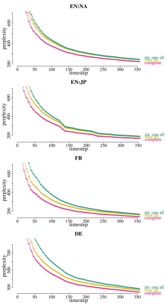
We can also see how the models performed over time. Figure 4 traces perplexity for four Reuters news stream datasets.13 We can see that in some cases the performance of the “base all” model degraded over time, whereas our model is more robust to temporal
13In both experiments, in order to manage the time and space
complexities of updatingβ, we apply a sparsity shrinkage
tech-nique by using OWL-QN (Andrew and Gao, 2007) when maxi-mizing it, with regularization constant set to 1. Intuitively, this is equivalent to encouraging the deviation vector to be sparse (Eisenstein et al., 2011).
shifts.
In the bigram experiments, we only ran our model with c = 7, since we need to maintainβ in RV2
, instead ofRV in the unigram model. The goal of
this experiment is to determine whether our method still adds benefit to more expressive language mod-els. Note that the weights of the linear interpolation models are also learned in an online fashion since there are no classical training, development, and test sets in our setting. Since the “base one” model per-formed poorly in this experiment, the performance of the interpolated models also suffered. For example, the “int. one all” model needed time to learn that the “base one” model has to be downweighted (we started with all interpolated models having uniform weights), so it was not able to outperform even the “base all” model.
6.4 Analysis and Discussion
It should not be surprising that conditioning on world-context reduces perplexity (Cover and Thomas, 1991). A key attraction of our model, we believe, lies in the ability to inspect its parameters.
Twitter:Google
timestep
β
0 100 200 300 400 500 600
0.0
0.5
1.0
1.5
2.0
goog goog
@google @google google+ google+ #goog #goog
rGOOG rGOOG
Twitter:Microsoft
timestep
β
0 100 200 300 400 500 600
0.0
0.5
1.0
1.5
[image:9.612.74.540.61.184.2]microsoft microsoft msft msft #microsoft #microsoft rMSFT rMSFT
Figure 3: Deviation coefficientsβover time for Google- and Microsoft-related words on Twitter with unigram base model (c= 7). Significant changes (increases or decreases) in the returns of Google and Microsoft stocks are usually followed by increases inβof related words.
investigate the deviations learned by our model on the Twitter dataset. Examples are shown in Figure 3. The left plot showsβ for four words related to Google:
goog,#goog,@google,google+. For compari-son, we also show the return of Google stock for the corresponding timestep (scaled by 50 and centered at 0.5 for readability, smoothed using loess (Cleveland, 1979), denoted byrGOOGin the plot). We can see that significant changes of return of Google stocks (e.g., therGOOGspikes between timesteps 50–100, 150–200, 490–550 in the plot) occurred alongside an increase inβ of Google-related words. Similar trends can also be observed for Microsoft-related words in the right plot. The most significant loss of return of Microsoft stocks (the downward spike near timestep 500 in the plot) is followed by a sudden sharp increase inβof the words#microsoftand
microsoft.
Feature coefficients. We can also inspect the learned feature coefficientsα to investigate which stocks have higher associations with the text that is generated. Our feature coefficients are designed to reflect which changes (or lack of changes) in stock prices influence the word distribution more, not which stocks are talked about more often. We find that the feature coefficients do not correlate with obvious company characteristics like market capi-talization (firm size). For example, on the Twitter dataset with bigram base models, the five stocks with the highest weights are: ConAgra Foods Inc., Intel Corp., Bristol-Myers Squibb, Frontier Communica-tions Corp., and Amazon.com Inc. Strongly negative weights tended to align with streams with less
activ-time lags
fre
que
nc
y
0
20
40
60
80
1 2 3 4 5 6 7 8 9 10 11 12 13 14
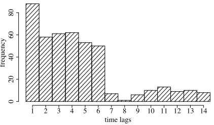
Figure 5: Distributions of the selection probabilities of models from the previousc= 14timesteps, on the EN:NA dataset with unigram base model. For simplicity, we show E-step modes. The histogram shows that the model tends to favor models from days closer to the current date.
ity, suggesting that these were being used to smooth across allcdays of history. A higher weight for stock oimplies an increase in probability of choosing mod-els from previous timestepss, when the state of the world for the current timesteptand timestepsis the same (as represented by our similarity function) with respect to stocko(all other things being equal), and a decrease in probability for a lower weight.
Selected models. Besides feature coefficients, our model captures temporal shift by modeling similar-ity across the most recentcdays. During inference, our model weights different word distributions from the past. The similarity is encoded in the pairwise featuresf(xt,xk)and the parametersα. Figure 5
[image:9.612.320.531.256.380.2]EN:NA
timestep
pe
rpl
exi
ty
0 50 100 150 200 250 300 350
200
400
600
base all base all complete complete int. one all int. one all
EN:JP
timestep
pe
rpl
exi
ty
0 50 100 150 200 250 300 350
200
400
600
base all
base all
complete
complete
int. one all
int. one all
FR
timestep
pe
rpl
exi
ty
0 50 100 150 200 250 300 350
200
400
600
base all base all complete
complete
int. one all
int. one all
DE
timestep
pe
rpl
exi
ty
0 50 100 150 200 250 300 350
300
500
700
base all
base all complete complete
int. one all
[image:10.612.143.469.69.669.2]int. one all
in the past they are at the time of use, aggregated across rounds on the EN:NA dataset, for window size c= 14. It shows that the model tends to favor models from days closer to the current date, with thet−1 models selected the most, perhaps because the state of the world today is more similar to dates closer to today compare to more distant dates. The plot also explains why increasingcfrom 7 to 14 did not im-prove performance of the model, since most of the variation in our datasets can be captured with models from the past week.
Topics. Latent topic variables have often figured heavily in approaches to dynamic language model-ing. In preliminary experiments incorporating single-membership topic variables (i.e., each document be-longs to a single topic, as in a mixture of unigrams), we saw no benefit to perplexity. Incorporating top-ics also increases computational cost, since we must maintain and estimate one language model per topic, per timestep. It is straightforward to design mod-els that incorporate topics with single- or mixed-membership as in LDA (Blei et al., 2003), an in-teresting future direction.
Potential applications. Dynamic language models like ours can be potentially useful in many applica-tions, either as a standalone language model, e.g., predictive text input, whose performance may de-pend on the temporal dimension; or as a component in applications like machine translation or speech recognition. Additionally, the model can be seen as a step towards enhancing text understanding with numerical, contextual data.
7 Conclusion
We presented a dynamic language model for stream-ing datasets that allows conditionstream-ing on observable real-world context variables, exemplified in our ex-periments by stock market data. We showed how to perform learning and inference in an online fashion for this model. Our experiments showed the predic-tive benefit of such conditioning and online learning by comparing to similar models that ignore temporal dimensions and observable variables that influence the text.
Acknowledgements
The authors thank several anonymous reviewers for help-ful feedback on earlier drafts of this paper and Brendan O’Connor for help with collecting Twitter data. This re-search was supported in part by Google, by computing resources at the Pittsburgh Supercomputing Center, by National Science Foundation grant IIS-1111142, AFOSR grant FA95501010247, ONR grant N000140910758, and by the Intelligence Advanced Research Projects Activ-ity via Department of Interior National Business Center contract number D12PC00347. The U.S. Government is authorized to reproduce and distribute reprints for Govern-mental purposes notwithstanding any copyright annotation thereon. The views and conclusions contained herein are those of the authors and should not be interpreted as nec-essarily representing the official policies or endorsements, either expressed or implied, of IARPA, DoI/NBC, or the U.S. Government.
References
Galen Andrew and Jianfeng Gao. 2007. Scalable training
ofl1-regularized log-linear models. InProc. of ICML.
David M. Blei and John D. Lafferty. 2006. Dynamic topic models. InProc. of ICML.
David M. Blei, Andrew Y. Ng, and Michael I. Jordan. 2003. Latent Dirichlet allocation. Journal of Machine Learning Research, 3:993–1022.
S´ebastien Bubeck. 2011. Introduction to online opti-mization. Technical report, Department of Operations Research and Financial Engineering, Princeton Univer-sity.
Nicol`o Cesa-Bianchi and G´abor Lugosi. 2006.Prediction, Learning, and Games. Cambridge University Press. William S. Cleveland. 1979. Robust locally weighted
regression and smoothing scatterplots. Journal of the American Statistical Association, 74(368):829–836. Thomas M. Cover and Joy A. Thomas. 1991.Elements of
Information Theory. John Wiley & Sons.
John Duchi and Yoram Singer. 2009. Efficient online and batch learning using forward backward splitting.
Journal of Machine Learning Research, 10(7):2899– 2934.
Jacob Eisenstein, Brendan O’Connor, Noah A. Smith, and Eric P. Xing. 2010. A latent variable model for geographic lexical variation. InProc. of EMNLP. Jacob Eisenstein, Amr Ahmed, and Eric P. Xing. 2011.
Sparse additive generative models of text. InProc. of ICML.
Matt Hoffman, David M. Blei, Chong Wang, and John Paisley. 2013. Stochastic variational inference. Jour-nal of Machine Learning Research, 14:1303–1347. Antti Honkela and Harri Valpola. 2003. On-line
varia-tional Bayesian learning. InProc. of ICA.
Tomoharu Iwata, Takeshi Yamada, Yasushi Sakurai, and Naonori Ueda. 2010. Online multiscale dynamic topic models. InProc. of KDD.
Frederick Jelinek. 1997. Statistical Methods for Speech Recognition. MIT Press.
Jyrki Kivinen and Manfred K. Warmuth. 1997. Expo-nentiated gradient versus gradient descent for linear predictors.Information and Computation, 132:1–63. Victor Lavrenko, Matt Schmill, Dawn Lawrie, Paul
Ogilvie, David Jensen, and James Allan. 2000. Mining of concurrent text and time series. InProc. of KDD Workshop on Text Mining.
Abby Levenberg and Miles Osborne. 2009. Stream-based randomised language models for SMT. In Proc. of EMNLP.
Abby Levenberg, Chris Callison-Burch, and Miles Os-borne. 2010. Stream-based translation models for sta-tistical machine translation. InProc. of HLT-NAACL. Dong C. Liu and Jorge Nocedal. 1989. On the limited
memory BFGS method for large scale optimization.
Mathematical Programming B, 45(3):503–528. David Mimno and Andrew McCallum. 2008. Topic
mod-els conditioned on arbitrary features with Dirichlet-multinomial regression. InProc. of UAI.
Alexander Rakhlin. 2009. Lecture notes on online learn-ing. Technical report, Department of Statistics, The Wharton School, University of Pennsylvania.
Masaaki Sato. 2001. Online model selection based on the variational bayes. Neural Computation, 13(7):1649– 1681.
Shai Shalev-Shwartz. 2012. Online learning and online convex optimization. Foundations and Trends in Ma-chine Learning, 4(2):107–194.
Martin J. Wainwright and Michael I. Jordan. 2008. Graph-ical models, exponential families, and variational infer-ence. Foundations and Trends in Machine Learning, 1(1–2):1–305.
Chong Wang, David M. Blei, and David Heckerman. 2008. Continuous time dynamic topic models. InProc. of UAI.
Chong Wang, John Paisley, and David M. Blei. 2011. On-line variational inference for the hierarchical Dirichlet process. InProc. of AISTATS.