Nonparametric Analysis of the
Order-Statistic Model in Software Reliability
Simon P. Wilson and Francisco J. Samaniego
Abstract—In the literature on statistical inference in software reliability, the assumptions of parametric models and random sampling of bugs have been pervasive. We argue that both assumptions are problematic, the first because of robustness concerns and the second due to logical and practical difficulties. These considerations motivate the approach taken in this paper. We propose a nonparametric software reliability model based on the order-statistic paradigm. The objective of the work is to estimate, from data on discovery times observed within a type I censoring framework, both the underlying distributionFfrom which discovery times are generated andN, the unknown number of bugs in the software. The estimates are used to predict the next time to failure. The approach makes use of Bayesian nonparametric inference methods, in particular, the beta-Stacy process. The proposed methodology is illustrated on both real and simulated data.
Index Terms—Beta-Stacy process, order statistics, reliability, testing strategies, nonparametric statistics, survival analysis.
Ç
1
I
NTRODUCTIONS
OFTWARE reliability models have received a lot ofattention in recent decades, as software systems have become more pervasive and vital to the operation of many important aspects of modern life. These models attempt to describe the process of bug discovery in software, typically in the prerelease stage of software development, when the software is tested to ensure that it meets its specification and to remove errors. Among their important purposes is predicting the total number of errors that will be discovered in the code and optimizing the software development process, for example, deciding on optimal testing strategies and when to release software for use.
The data usually take the form of times between bug discoveries or counts of discovered bugs at known times. The structure of the data, and so a reasonable model for them, is very dependent on the type of software, the use to which the software is put, and the circumstances under which the data were collected. Because of this, a plethora of parametric models, based on many different modeling approaches and ideas about the structure of the data, have arisen that work well for certain data but lack robustness.
In this paper, we investigate one common class of software reliability model—the order-statistic model—and, in doing so, attempt to address the problem of achieving a better flexibility in the modeling approach. We also point out a deficiency in the sampling scheme that most software reliability models assume and offer a more reasonable
alternative. We consider a nonparametric approach on the basis that this provides the desired robustness in modeling. Bayesian inference is developed that infers the posterior distribution of the discovery time distribu-tions and the number of bugs and is illustrated on real and simulated data. Once this is done, we show how the estimates may be used to predict next time to failure. As well as describing methodology for this class of models, we believe that it is an interesting extension of Bayesian nonparametric approaches.
Order-statistic models assume that there are an un-known number of bugsNin the software. Bugs are labeled i¼1;. . .; N and their discovery times are independent, specified by distribution functions G1; G2;. . .; Gn. The
observed sequence of discovery times are the order statistics of the Gi. The earliest order-statistic model for
software reliability is the Jelinski-Moranda model [1], which assumes that the Gi are independent and identically
distributed exponential random variables, although the authors did not categorize the model as of that type. The order-statistic model approach was first defined for use in software reliability in [2], although the idea was implicit in the earlier work of [3]. Here, the Gi were exponential
(making the work of [1] a special case) but not necessarily identically distributed, equivalent to assuming that each bug failed as an independent Poisson process. There had been some work on order-statistic models in general reliability theory beforehand; see [4]. A more general order-statistic model, that moved beyond the exponential assumption was proposed in [5].
A feature of all these papers is that a parametric form for the Gi is assumed. Our work attempts to generalize to a
nonparametric form for theGi. However, in order to make
inference practical, we work with a special case, where the Giare identical; we explain why in Section 2. The work of [6]
is the closest that we have found to our approach, where the general order-statistic model is treated nonparametrically. . S.P. Wilson is with the Department of Statistics, Trinity College Dublin,
Dublin 2, Ireland. E-mail: [email protected].
. F.J. Samaniego is with the Department of Statistics, University of California at Davis, One Shields Avenue, Davis, CA 95616.
E-mail: [email protected].
Manuscript received 31 July 2006; accepted 7 Dec. 2006; published online 26 Jan. 2007.
Recommended for acceptance by B. Littlewood.
When N is assumed known, inference for an order-statistic model is typically straightforward. When N is unknown, as is the case with software testing data, the inference is a type of “how many kinds are there” problem, well-known in the literature on estimating numbers of distinct species. It is pointed out in [7] that, in some cases, the data contain little information aboutN; thus, inference can be more difficult. In this regard, a Bayesian approach has the advantage that it can make use of any prior knowledge aboutN to aid the inference. In [8], a Bayesian approach was described for an example of an exponential order-statistic model. For the general order-statistic model, inference procedures are described in [9] and [5], while [10] is an example of Bayesian inference.
There have been previous applications of Bayesian nonparametric methods in software reliability, but they have been restricted to a hierarchical semiparametric approach, where a parametric model for the discovery times is assumed, and a nonparametric model is assigned for the prior on a model parameter; see [11] and [12]. The approach is also related to work in warranty analysis, where the failure of systems under warranty is analyzed; see [13].
The paper is organized as follows: In Section 2, we define the order-statistic model and demonstrate the problems that can arise for inference when a parametric form of the model is assumed. In Section 3, we define the nonparametric form of the order-statistic model and describe a Bayesian inference procedure for the distribution function from which the discovery time distribution is defined and N, the number of bugs. Section 4 discusses how to present the inference and how to apply it to prediction. Section 5 gives examples using simulated and real data. In Section 6, we close with some concluding remarks.
2
A N
ONPARAMETRICO
RDER-S
TATISTICM
ODEL We assume that software has an unknown number N of bugs and is being tested. We denote the bug discovery times asT1;. . .; Tnand they are the order statistics of a set of N independent random variables with distribution func-tionsG1;. . .; GN. Defining the distribution functions of the Ti to be FiðtÞ, standard order-statistic theory defines the FiðtÞ in terms of the GiðtÞ and N; see [14]. For example,letting GiðtÞ ¼1et,t0,8i, it is shown in [2] that we
have the well-known Jelinski-Moranda model [1], where
Fiðtj; NÞ ¼1expððNiþ1ÞtÞ: ð1Þ
The model that we define and explore in this paper is a general order-statistic model, but the Gi are not defined
parametrically. It is a very flexible extension to the Jelinski-Moranda model; theGiare identical but are not given any
parametric form. We letGiðtÞ ¼FðtÞ,8i; hence, our model
is defined byFðtÞandN.
Assuming a commonF is a simplifying approximation, but we argue that the model is still useful—when the data model is in an appropriate neighborhood of the Jelinski-Moranda model, for example—and is a stepping stone to thinking about more complex nonparametric models. Indeed, without some assumption to link the Gi, a
nonparametric analysis is a hopeless proposition. The
assumption of identical Gi allows us to implement an
MCMC scheme for Bayesian inference. So, our work can be considered as a nonparametric generalization of the Jelinski-Moranda model or as a general order-statistic model with identical nonparametric discovery time dis-tribution. We note that the nonparametric distribution can be multimodal, allowing one to think of the bugs as coming from separate subpopulations.
2.1 The Random Sampling Scheme
The usual assumption is that data consist of a set of k independent interdiscovery times t1;. . .; tk, where k is
fixed, having likelihood
Lð; Njt1;. . .; tkÞ ¼
Yk
i¼1
fiðtijN; Þ;
wherefiðtijN; Þ ¼Fi0ðtijN; Þis the density function of the ith interdiscovery time, parameterized by . We observe that a fixed and predetermined choice ofkimplies that one has assumed that N k. This assumption is, in general, both risky and impossible to justify and runs counter to the experimenter’s natural inclination to sample as many bugs as possible, both because so doing improves the software, through the removal/repair of the discovered bugs, and because the precision of one’s estimates of model para-meters tends to improve as the sample size increases.
Because of the tenuous nature of the “fixedk” assump-tion, we propose a type I censoring framework, where the software is observed for a fixed predetermined amount of timeT. The protocol for bug discovery and removal is the same as that discussed above. A consequence of this alternative model is that the numberkof bugs discovered in the time interval ð0; TÞ is a nonnegative random variable. Whilek can take on the value zero with positive probability, this probability is negligibly small in most applications of interest. This leads toNkdiscovery times to be right-censored atT.
This is a more appropriate and realistic framework for sampling software bugs than the fixed sample-size ap-proach. Assume that the discovery times are independent with distribution function F and density f. We view our data to consist of bothkandt1;. . .; tk. GivenN andF, the
number of discovery times k before T is binomial with probability parameter FðTÞ. Given k and T , the order-statistic model gives the distribution oft1;. . .; tk to be the
joint order statistics distribution of a sample of sizekfrom F, given thatti< T. Given this, we arrive at the likelihood
for these data:
LðF ; NjT; k; t1;. . .; tkÞ
¼Pðt1;. . .; tk; kjT; N; FÞ ¼Pðt1;. . .; tkjT; k; N; FÞPðkjT; N; FÞ
¼ k!Y k
i¼1 fðtiÞ FðTÞ
" #
N k FðT
Þk
ð1FðTÞÞNk
¼ N!
ðNkÞ!ð1FðT
ÞÞNkYk
i¼1 fðtiÞ;
2.2 Parametric Models
Parametric models for bug counting schemes have been shown to have some undesirable properties and can lack robustness. In particular, most of the models assume reliability growth, and if the data do not clearly demon-strate this, then maximum likelihood estimates of N can become infinite; see [15]. The problems that can occur with the Jelinski-Moranda model in this regard are described in [16].
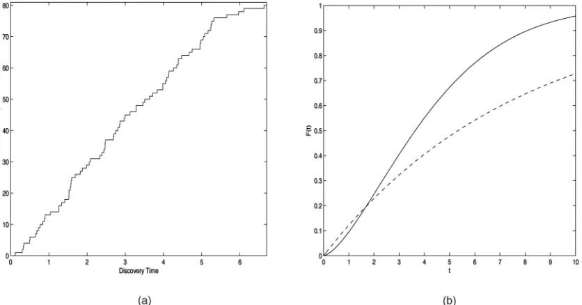
To illustrate this lack of robustness of the parametric bug counting model, we fit the Jelinski-Moranda model to a simulated data set ofk¼80discovery times, withT¼6:7
(t80¼6:63 being the final discovery time) from a Weibull
order-statistic model withN ¼100and
FðtÞ ¼1expð0:1t1:5Þ;
thus, FiðtÞ ¼1expð0:1ð101iÞt1:5Þ. The data are
dis-played in Fig. 1a. The maximum likelihood estimate for the Jelinski-Moranda model, for which FðtÞ ¼1expðtÞ, is found numerically to beðN;^ ^Þ ¼ ð137; 0:13Þ. The estimated
FðtÞ ¼1expð0:13tÞ is plotted in Fig. 1b, along with the true F, and we see that the true F has been very badly estimated, even though this particular Weibull is only modestly different from the Jelinski-Moranda model, where F is an exponential distribution.
3
B
AYESIANN
ONPARAMETRICA
NALYSISIn this section, we describe a Bayesian inference procedure that computes the posterior distribution ofF andN from discovery time data under the type I censoring scheme of Section 2.
A Bayesian analysis requires a likelihood and prior distribution for F and N. Given our model in terms ofF andN, application of the expression for the likelihood in (2) gives us a likelihood
LðF ; Njt1;. . .; tk; TÞ
¼ N!
ðNkÞ!ð1FðT
ÞÞNkY
k
i¼1
ðFðtiÞ FðtiÞÞ; ð3Þ
where we have replaced the probability densityfðtiÞ with
the termFðtiÞ FðtiÞ, referring to the limit from the left,
appropriate where there is a point mass atti.
For a prior distribution, we assume that N and F are independent a priori. This is principally for mathematical convenience. However, a priori dependence betweenNand F may be desirable since, if N increases as the expected value ofF increases, we may model the same beliefs about the discovery times. Thus, positive dependence betweenN and the expected value of F may be appropriate. In practice, we will assume rather flat, noninformative priors that we show have little effect on the posterior distribution.
3.1 Prior Specification forN
Several techniques have been proposed for specifying a prior forN in the context of bug counting, for example, the use of software metrics [17] or the use of elicitation techniques [18]. In these cases, analysis of the sensitivity of the posterior to the prior on N will be essential. One might also use noninformative proper priors, such as discrete uniform on a finite range f0;. . .; Nmaxg, where Nmaxis a suitably chosen upper bound, such as the number
of characters in the code.
3.2 Prior Specification forF
The usual prior distribution on the set of possible distribu-tion funcdistribu-tions is the Dirichlet process prior [19]. It is a distribution over the set of all discrete distribution functions and is defined by a finite measureon the sample space, which is the expected value of the prior. The expected distribution has measure=ðIRÞ. If the datax1;. . .; xn are
[image:3.612.78.496.69.288.2]ðIRÞcontrols the relative importance that is placed on the prior; by making this small, the posterior will be dominated by the data.
Inspired by the Jelinski-Moranda model, we assume that the mean of the prior model is the exponential distribution with failure rate; thus,ðtÞ ¼Bet, forB >0, whereB¼ ðIRÞis the prior weight. We may then specify a hyperprior distribution for or assign it a value. Here, we adopt an empirical Bayes approach and specifyto be the MLE of the Jelinski-Moranda model. In our experience, the inference is not sensitive to the choice ofif one keeps the prior weight Bsmall relative tok.
3.3 The Posterior Distribution ofðN; FÞ
The objective of the Bayesian analysis is to compute the posterior distribution of F and N given t1;. . .; tk; T. This
is done by simulating values of F and N using Gibbs sampling. That is to say, we simulate a distribution function F from PðFjN; t1;. . .; tk; TÞ and then a value
of N from PðNjF ; t1;. . .; tk; TÞ. After repeated alternate
sampling of F and N from these distributions, the sampled F and N are from PðF ; Njt1;. . .; tk; TÞ. Below,
we describe how to sample from the two full conditional distributions.
3.4 Sampling from the Posterior Distribution of F GivenN
The key to being able to simulate a realization of F given N is to consider the data as purely observations from F. As we observed when defining (3), if N is known, then the order-statistic model that we propose allows us to interpret our data as k observations t1;. . .; tk from F and Nk observations right-censored at T. The presence of right-censored data means that the posterior distribution is no longer represented by a Dirichlet process but is of a more general form defined through a stochastic process called the beta-Stacy process; Walker et al. [20] discuss beta-Stacy processes in detail, and we refer the reader to that paper for a comprehensive description.
For our purposes, it is sufficient to know that the posterior of F can be written as FðtÞ ¼1expðZðtÞÞ, where ZðtÞ is a beta-Stacy process. Such processes have countably many points of discontinuity and can be written as the sum of independent increments W1; W2;. . . at those
discontinuity points and a continuous component. It is shown in [21] that, with a Dirichlet prior having measure ðtÞ and data observed at x1; x2;. . ., some of which may
be right censored, the posterior for F can be written FðtÞ ¼1expðZðtÞÞ, where
ZðtÞ ¼ZcðtÞ þ
X
i:xiuncensored
Iðxi< tÞWi; ð4Þ
whereIis the indicator function,ZcðtÞis a continuous Levy
process which they define (also see [21]), the jumpsWihave
density function
fiðwÞ / ð1ewÞNfxig1
exp w ðxiÞ þ
X
j
IðxjxiÞ Nfxig
" #!
; ð5Þ
and where Nfxig is the number of exact (noncensored)
observations atxi.
Our goal is to sample from this process. We will see that, to sample N, it is sufficient to compute F at the ti, i¼1;. . .; k, and T. Therefore, we sample the jumps W1;. . .; Wk that occur at t1;. . .; tk—there is no jump at T
because there is no uncensored observation—and sampleZc
between successive observations, e.g.,
Zcðt1Þ; Zcðt2Þ Zcðt1Þ;. . .; ZcðtkÞ Zcðtk1Þ
andZcðTÞ ZcðtkÞ, from which
ZcðtiÞ ¼Zcðt1Þ þ
Xi
j¼2
½ZcðtjÞ Zcðtj1Þ:
Then,FðtiÞandFðtiÞare given by
FðtiÞ ¼1expðZðtiÞÞ
¼1exp ZcðtiÞ
Xi1
j¼1 Wj
!
ð6Þ
and
FðtiÞ ¼1expðZðtiÞÞ
¼1exp ZcðtiÞ
Xi
j¼1 Wj
!
: ð7Þ
To sample the jumps, it is easy to sample from the distribution in (5). In most cases, all the t1;. . .; tk are
distinct, so Nftig ¼1 and the Wi are exponentially
distributed with a mean ½ðtiÞ þNi1. The sampling
of the continuous component is more complex, but follows exactly the developments in [21]. A Markov chain Monte Carlo method is needed; in fact, two chains are required for each sample of ZcðtiÞ Zcðti1Þ. For the
reader’s convenience, the sampling method is described in Appendix A.
3.5 Sampling from the Posterior Distribution of N GivenF
Given F, the full conditional distribution of N is by Bayes’ law:
PðNjF ; t1;. . .; tk; TÞ /LðF ; Njt1;. . .; tk; TÞPðNÞ
¼ N!
ðNkÞ!ð1FðT
ÞÞNk Yk
i¼1
ðFðtiÞ FðtiÞÞ
! PðNÞ
/ N!
ðNkÞ!ð1FðT
ÞÞN
PðNÞ; ð8Þ
forNk, with
1FðTÞ ¼exp ZcðTÞ
Xk
i¼1 Wi
!
¼exp
ðZcðt1Þ ðZcðTÞ ZcðtkÞÞ
X k
i¼2
ðZcðtiÞ Zcðti1ÞÞ
Xk
i¼1 Wi
hence, to sampleN it is sufficient to have sampled theWi
and Zc between successive discovery times and from tk to T, as described in the last Section 3.4.
We directly compute the probabilities of (8) and sample N by the inverse distribution function method.
3.6 MCMC Convergence
As with all MCMC methods, we must assess if the sampling method has converged. Lack of convergence is usually tested by plotting traces of the sampled quantities inF—the Wi and the continuous components ZcðtiÞ Zcðti1Þ—and N, by applying statistical tests for autocorrelations and other signs of nonconvergence. However, here the issue is complicated because each sampled component ZcðtiÞ Zcðti1Þ is itself computed from the output of two MCMC
chains (see Appendix A). A possibility is that we judge F andN to be sampled from a chain in equilibrium, but that this is from unconverged chains for the ZcðtiÞ Zcðti1Þ.
Further, given that2ðkþ1Þchains must be run to get each sample of F, it is impractical to go through each of these chains individually, looking for signs of nonconvergence.
We attempt to address this problem by running each of the chains required for ZcðtiÞ Zcðti1Þ for a different
randomly chosen number of iterations. An example is given in Appendix B, where the length of the first chain was chosen uniformly between 7,000 and 25,000 iterations; this pertains to a parameter that is denoted. The second chain samples a sequence of values denoted by 1;. . .; . This
chain was constructed by a uniformly random burn-in period between 5,000 and 50,000 iterations, and the number of iterations between each samplejwas uniformly chosen
between 2,000 and 15,000. Then the computed values of and ZcðtiÞ Zcðti1Þ are compared against the number of
iterations in the MCMC chain used to compute them. If the chain lengths are sufficient, we should see no relationship between number of iterations and the computed values. If we see no evidence from this test of nonconvergence or bad mixing, we proceed to look at the samples ofF andNin the usual way to test for nonconvergence.
4
D
ISPLAYING THEP
OSTERIOR OFF
, M
ODELF
IT, ANDP
REDICTINGT
IME TON
EXTD
ISCOVERY In this section, we describe how to display the posterior distribution in an informative manner, how to assess the performance of the fitted model, and how to use the posterior distribution of N and F that was simulated in Section 3 to compute the distribution of the next time to failure.We assume that L samples of FðtÞ and N have been generated. Let ðFðtÞðlÞ; NðlÞÞ be the lth sample from the
posterior distribution ofF andN. For each observed time, we estimate the posterior mean ofFðtiÞ andFðtiÞ as the
mean of the sampled values of FðtiÞ and FðtiÞ, for i¼ 1;. . .; k using (6) and (7). Estimates of FðtÞ between observation times are obtained by linear interpolation of ZðtÞ. Similarly, taking high and low percentiles of the FðtiÞðlÞ gives upper and lower bounds to the posterior at
each observed time.
Model evaluation is done by comparing the observed failure times with estimates of its distribution. The
ith observed discovery time ti is the ith order statistic
from an independent sample of sizeN with distributionF. Hence,
FiðtÞ ¼
XN
j¼i N
j FðtÞ j
ð1FðtÞÞNj;
from which an obvious predicted value is the posterior median. We compare this posterior median withti. For each
sample of FðtÞ and N, we compute its ith order statistic distribution:
FiðtÞðlÞ¼
XNðlÞ
j¼i NðlÞ
j
½FðtÞðlÞjð1FðtÞðlÞÞNðlÞj:
By interpolating between theti, any percentile ofFiðtÞðlÞcan
be computed; we denote the 100 percentile as Fi;ðlÞ. The
posterior mean of the100percentile of the distribution of theithobserved discovery time can be computed by
Fi; 1
L XL
l¼1
Fi;ðlÞ: ð9Þ
The median is calculated from (9) with ¼0:5. A prediction interval for the ith discovery time is then the 2.5 percent and 97.5 percent points of the posterior distribution of FiðtÞ, again calculated by (9). Because of
the right censoring in the data, we may not estimateFiðtÞ
well in the right tail. This feature is quite familiar in nonparametric estimation; for example, the Kaplan-Meier estimator of an underlying survival function never attains the value zero when the largest observation is a censored failure time. This is particularly the case fori neark, and more so if the posterior distribution of N places large probability close tok.
The distribution of the discovery time of the next bug is the ðkþ1Þth order statistic, left-truncated at T since
we did not observe it by this time. If N ¼k, then there are no more bugs to be discovered and Tkþ1¼ 1 with
probability 1. We define this in terms of the reliability functionFkþ1ðtjTkþ1TÞ ¼1F
kþ1ðtjTkþ1TÞ:
Fkþ1ðtjTkþ1TÞ ¼
1Fkþ1ðtÞ 1Fkþ1ðTÞ
¼
Pk j¼0
N j ð ÞFðtÞj
ð1FðtÞÞNj
Pk j¼0
N j ð ÞFðTÞj
ð1FðTÞÞNj if Nkþ1;
1; ifN ¼k;
8 > < > : ð10Þ
for tT, which we compute in a similar way to the
computation ofFðtÞ. For thelthsample, we compute
Fkþ1ðtjTkþ1TÞðlÞ¼1
ifNðlÞ¼kand
Fkþ1ðtjTkþ1TÞðlÞ
¼
Pk j¼0
NðlÞ
j
½FðtÞðlÞjð1FðtÞðlÞÞNðlÞj
Pk j¼0
NðlÞ
j
½FðTÞðlÞ
ifNðlÞkþ1. We then take the mean of theFkþ1ðtÞðlÞas our
estimate of Fkþ1ðtjTkþ1TÞ. Uncertainty in F
kþ1ðtÞ is
described by looking at percentiles of theFkþ1ðtÞðlÞ, e.g., the
2.5th and 97.5th percentiles provides a 95 percent prob-ability interval. Since Fkþ1ðtÞ ¼1; 8t with probability PðN¼kjt1;. . .; tk; TÞ, the100percentile of the posterior
distribution of Fkþ1ðtÞ will be 1,
8PðN ¼kjt1;. . .; tk; TÞ:
In practice, we find the inference easier to interpret if we report PðN ¼kjt1;. . .; tk; TÞ and Fkþ1ðtÞ conditional on N kþ1, where we only consider samples for which NðlÞ> k, e.g., the posterior mean is
Fkþ1ðtjTkþ1T; Nkþ1Þ 1
jfljNðlÞ> kgj
X
l:NðlÞkþ1
Fkþ1ðtjTkþ1TÞðlÞ;
tT:
Note that, to estimateFkþ1, we require samples ofFðtÞðlÞfor t > T. We only sampled values of F up to t¼T in Section 3, so to do this, we need to generate a sample of the beta-Stacy processZðtÞfort > T. Since the Gibbs sampler
of Section 3 gives us samples of ZðTÞ and there are no jumps in the beta-Stacy process fort > T—they only occur att1;. . .; tk—what is required is to simulate the continuous
part of the process fromTtot. This we do in the manner of Section 3 for as many different values oftas we require.
5
E
XAMPLES5.1 Simulated Weibull Data
[image:6.612.299.525.67.464.2]To see how well the inference procedure works, it is applied to the simulated Weibull data described in Section 2.2 and Fig. 1. The maximum likelihood estimate from the Jelinski-Moranda model for these data is ð;^N^Þ ¼ ð0:13;137Þ. The prior onFis therefore taken to be Dirichlet with mean as an exponential distribution with ¼0:13 and a small weight B¼1. A uniform prior onf0;1;. . .;1;000gis placed onN. Ten thousand samples ofN andF were generated. The convergence of the chains was assessed using the ideas of Section 3.6. The assessment showed no signs of nonconver-gence, and we determined adequate chain lengths for the sampling ofto be 100,000 iterations, while for thej, there
was a burn-in of 20,000 iterations, with successive jtaken
every 10,000 iterations. Details of how the chain lengths are determined are in Appendix B.
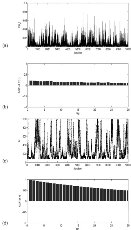
Fig. 2 shows the sampled values and autocorrelation function of Fðt1Þ and N, respectively. The chain forFðt1Þ
shows good mixing and no sign of nonconvergence. It is typical of those for other FðtiÞ. However, the sampled
values forN are not as well behaved and show persistent autocorrelation. This is due to the very long tail in the distribution of N that the Gibbs sampler takes time to explore. It is clear that the prior upper bound toN of 1,000 has truncated the posterior distribution.
Fig. 3 shows the posterior distribution ofF, as described in Section 4, and a histogram of the sampled values of N. The plot of F also shows the Weibull distribution that generated the data and the Kaplan-Meier estimate for F
given that we assume N¼100 (the true value). We note that the true F lies within the pointwise posterior probability interval forF, although the posterior mean for F is not close to the true F. However, we note that our mean estimate for F is very close to the Kaplan-Meier estimate, but that the latter is constructed given the true value of N. The posterior median of N is 180 and the posterior (2.5 percent, 97.5 percent) interval is (82, 913). The posterior mean is estimated to be 281. The true value ofNis the 18th percentile of the sampled values.
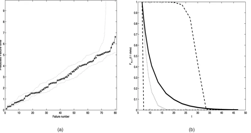
Further, in Fig. 4a, we compare the observed values with the predicted, and we see that the model has made good predictions of the observed values. In Fig. 4b is the prediction for the reliability function of the time to next failure, R81ðtÞ ¼ ð1FðtÞÞN80, conditional onN81. In this case,
we estimatePðN ¼80jdataÞ ¼0:008. This plot also shows the lower and upper 10th percentile of R81ðtÞ, the true
Weibull reliability function from which the data were generated and the Jelinski-Moranda F (the prior). We see that the estimated function overestimates the true reliability
Fig. 2. (a) The sampled values of Fðt1Þ. (b) Their autocorrelation
from the simulated model R81ðtÞ ¼expð1:5t1:5Þ, which is
mainly due to the underestimation of N, but that the true function lies well within the prediction bounds.
We also assessed the robustness of the posterior ofF to the value of . Setting ¼1:0, we saw that, in spite of the large misspecification, the posterior ofF was not different. The small value of B has ensured that the results are insensitive to the choice of prior distribution parameter.
This example shows that the model has fitted the data well (Fig. 4a); in particular, we have estimatedFto be close to the Kaplan-Meier estimate given the trueN. There is high
posterior variance in bothF and N (Fig. 3), the price that one pays for adopting such a general model. The posterior distribution ofNis sensitive to the choice of prior. However, experimentation showed that the model fit and reliability prediction (as in Fig. 4) were not sensitive to the upper bounds on the uniform prior that were higher than 1,000.
5.2 The NTDS Data
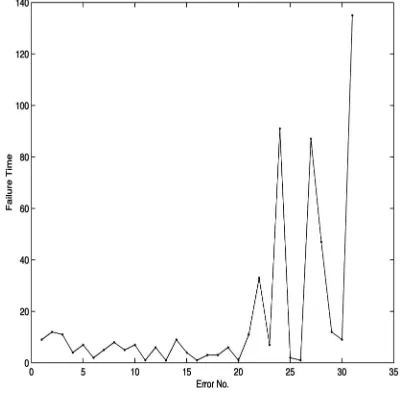
[image:7.612.78.491.68.289.2]The Naval Tactical Data System was a large software project for the US Navy. Data on the times of bugs detected in the testing phase of one of the modules form the NTDS data set, which originally appeared in [1].
Fig. 3. Analysis of the Weibull order-statistic simulated data. (a) The true and posteriorFðtÞ: pointwise posterior mean (thick solid line), pointwise posterior 2.5 and 97.5 percentiles (thin solid lines) and trueF(dashed line) and the Kaplan-Meier estimate ofFðtÞgiven the true valueN¼100 (dotted line). (b) A relative histogram of posterior samples ofN(grouped in intervals of 20).
[image:7.612.79.497.497.718.2]Fig. 5 displays the firstk¼31discovery times in the data, with T¼600 (t31¼540:0 being the final discovery time).
[image:8.612.51.253.71.271.2]The MLE in this case isðN;^ ^Þ ¼ ð31;0:0064Þ. The prior onF is assumed to be a Dirichlet process with exponential distribution mean having ¼0:0064, and a small weight B¼1. A uniform prior onf0;1;. . .;200gwas placed onN. The MCMC was run for 10,000 iterations. Fig 6a shows the estimated posterior ofF along with the prior, which is also the MLE estimate from the JM model. The prior and the posterior agree quite closely. Fig. 6b shows the sampled values of N. The posterior median of N is 31, and the (2.5 percent, 97.5 percent) probability interval is (31, 32). The posterior mean is 31.1. Moving to model assessment, Fig. 7a shows the predicted discovery times with the observed, as described in Section 4. It shows that, once again, the posterior distribution function has predicted well the observed discovery times.
Fig. 7b shows the posterior reliability function
R32ðtÞ ¼1F32ðtÞ ¼ ð1FðtÞÞN31:
The posterior probability thatN¼31(that is, that there are no further failures) is 0.94. The distribution compares well with the most recently observed discovery times and, in this case, agrees well with the reliability fitted from the JM model. Again, we see that the mean estimate for RKþ1ðtÞ
performs well, although there is considerable uncertainty in the estimate. The MLE from the JM model isN^¼k¼31, so it predicts that there are no new failures.
6
D
ISCUSSIONIn this paper, we have presented a Bayesian nonparametric approach to the treatment of bug discovery time data. We have argued that the assumption of a parametric model leaves the investigator vulnerable to the consequences of model misspecification. For the same reasons that the empirical distribution function or the Kaplan-Meier esti-mator might be preferred to a parametric alternative, one might well prefer a nonparametric analysis in assessing the reliability of a piece of software. The model is a nonpara-metric form of the order-statistic model. The inferential approach presented here has the natural robustness of a nonparametric analysis and has, as well, the ability to incorporate, through the modeling of prior information, pertinent intuition or expert knowledge that might be available in the application of interest.
The approach we have taken has consciously eschewed the “random sampling” assumption that is typical of traditional treatments of the estimation problem under study. Our developments assume, instead, that the software being tested is subjected to such testing over a fixed and predetermined interval of time. Under this type I censoring scheme, the number of bugs found is a random variable, and the inference developed is based on the random discovery times between the (random) number of bugs found.
Fig. 5. The NTDS data set.
[image:8.612.82.494.513.738.2]The approach presented in Sections 3 through 5 requires that the tester specify a prior distribution for N and a distribution function that is the mean of the prior for F, and we have suggested how these can be defined. The computation of the posterior distribution and pre-sentation of results can be complicated, but we have successfully demonstrated its feasibility in the examples presented herein.
The strengths of this approach are the more realistic sampling scheme and a more robust fitting procedure. The disadvantages are a complicated computation process, and the problem of evaluating convergence of the many separate Markov chains in the simulation procedure. Other criticisms are the assumption that the distributions gen-erating the order statistics are identical and that we have not modeled a priori dependence betweenF andN.
The former criticism is more difficult to address than the latter. If one allowed each bug to have a possibly differentF, then there would be one datum available to learn about each. The success of the inference relies on being able to treat all the observations as coming from one distributionF. Any model that relaxed the identical distribution assumption and wanted to make use of the method described here would have to allow the data to be treated in this way. We also point out that our modeling ofF allows it to be multimodal and, thus, describe a mixture of subpopulations of bugs.
Modeling dependence between N and F is more straightforward; for example, one could allow the expected value of the mean of F to depend on N. An obvious extension of the work is a fully Bayesian approach, where inference is also conducted on the parameters of the prior mean of F. The problem is that it is difficult to write the likelihood in terms of these parameters. Another extension is to fit count data rather than discovery times, by using data augmentation to sample times from a sample of F conditional on the counts.
The developments in this paper provide a useful stepping stone for facilitating further research on nonpara-metric software reliability. As with any Bayesian analysis,
we should mention the need to tailor the analysis to the intended application. A sensitivity analysis within any given application, so as to determine the extent to which the analysis is affected by the prior model, is important (see chapter 6 of [22]). One can present a Bayesian analysis with greater conviction when the inference is fairly stable over a class of “reasonable” prior distributions than when it is quite sensitive to the prior selected within such a class.
A
PPENDIXA
S
AMPLING FROMZ
cðt
iÞZ
cðt
i1Þ
Let there be a Dirichlet process prior forFwith measureðsÞ. Our data consist of noncensored observations at t1;. . .; tk
and Nk right-censored observations at T. In [21], it is
shown that the posterior distribution forFcan be written in the formFðtÞ ¼1expðZðtÞÞ, whereZðtÞis a beta-Stacy process. As is described in Section 3,ZðtÞcan be written as the sum of independent increments W1;. . .; Wk at the
observed discovery times t1;. . .; tk and a continuous
component ZcðtÞ. In this appendix, we describe how to
sample fromZcðtiÞ Zcðti1Þ, fori¼1;. . .; k, the change in
the continuous component between successive discovery times. The description is also valid for sampling from ZcðTÞ ZcðtkÞ. The beta-Stacy process has independent
increments, and so these increases in the continuous process are independent.
DefineðsÞto be such thatðsÞ ¼Rs1dðuÞ. In this case, we have definedðsÞ ¼Bes, from whichdðsÞ ¼Besds.
From [21], in our case, the continuous part of the posterior processZcðtÞhas Levy measure
Kðz; tÞ ¼expðz ½ ðtÞ þNiþ1ÞdðtÞ
1ez : ð11Þ
[image:9.612.79.493.68.291.2]processPj¼1j, where, for small, the number of jumpsis
Poisson with mean
¼
Z 1
0
Z 1
0
ezðsÞðsÞIðz > ; t
i1< s < tiÞ
1ez dz ds ð12Þ
and the jumpsjare independent and come from a density
gðzÞ /Iðz > Þ
Rti
ti1expðz ½ ðsÞ þNiþ1ÞdðsÞ
1ez : ð13Þ
A sample fromZcðt1Þis obtained by this definition if we let t0¼0. The approximation converges toZcðtiÞ Zcðti1Þ as !0; practically, we can taketo be small. In [23], the error in this approximation as a function ofis discussed, which is of the order EðÞ< ðti1; tiÞ. In this paper, following
some exploration, we found that there was no difference in results for any <105; thus, we set, conservatively, ¼107.
In order to sample the compound Poisson process P
j¼1j, we first sample, then samplefrom the Poisson
with mean, and then independently sample1;. . .; from gðzÞ. Summing thej obtains the approximate sample from ZcðtiÞ Zcðti1Þ. This is independently repeated for i¼ 1;. . .; kand also forZcðTÞ ZcðtkÞ. For the latter case, (11),
(12), and (13) are still valid with ti1 replaced by tk, ti
replaced byTandNiþ1(in (11) and (13)) replaced by Nkþ1. In [23], it is shown how to draw a sample from and from gðzÞ. For our specific case, one would do the following (which follows exactly the Appendix of that paper):
1. Sampling for ZcðtiÞ Zcðti1Þ. This is done by a
Gibbs sampler on variablesðz; sÞ. Take initial values of the sampler to be zð0Þ> and t
i1< sð0Þ< ti; for
sampling ZcðTÞ ZcðtkÞ, we have tk< sð0Þ< T.
Iterationlþ1of the sampler that drawsðzðlþ1Þ; sðlþ1ÞÞ
givenðzðlÞ; sðlÞÞis then:
a. Sample zðlþ1Þ from an exponential distribution
with mean ½ðsðlÞÞ þNiþ11
restricted to
ð;1Þ. For samplingZcðTÞ ZcðtkÞ, the mean is ½ðsðlÞÞ þNkþ11.
b. Samplesðlþ1Þ by a Metropolis move. Propose a pointsfrom the densityfðsÞ /ðsÞrestricted to ti1< s < ti. Letsðlþ1Þ¼s with probability the
minimum of 1 and
expzðlþ1ÞhðsÞ ðsðlÞÞi;
otherwise,sðlþ1Þ¼sðlÞ.
c. Once many samples have been taken, the chain has converged, and L samples from the sta-tionary distribution are taken, then
1
L XL
l¼1
1
1expðzðlÞÞ
Z ti
ti1
expððsÞÞ
ðsÞ dðsÞ;
where the integral here is one-dimensional and
should be sufficiently well approximated by the
easier to compute Rtiti1dðsÞ=ðsÞ ðti1; tiÞ.
For samplingZcðTÞ ZcðtkÞ, we replaceti1by
tkandti byT.
2. Sampling fromgðzÞ.A sample z from gðzÞ can be obtained by a Gibbs sampling scheme over vari-ablesðz; u; sÞ. Initial values arezð0Þ> ,0< uð0Þ<1,
andti1< sð0Þ< ti; for sampling ZcðTÞ ZcðtkÞ we
have tk< sð0Þ< T. To draw ðzðlþ1Þ; uðlþ1Þ; sðlþ1ÞÞ
given ðzðlÞ; uðlÞ; sðlÞÞ:
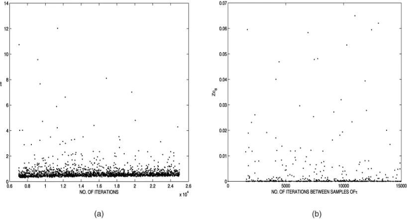
Fig. 8. (a) Sampled values offorZcðt28Þ Zcðt27Þagainst the number of iterations in the MCMC chain used to produce that value. (b) Sampled
[image:10.612.80.489.70.290.2]a. Sample zðlþ1Þ from an exponential distribution with mean ½ðsðlÞÞ þNiþ11
restricted to
ð;1ÞifuðlÞ1, or restricted to
ð;logð1 ðuðlÞÞ1Þ;
if uðlÞ>1. For sampling Z
cðTÞ ZcðtkÞ, the
mean is
½ðsðlÞÞ þNkþ11:
b. Sampleuðlþ1Þfrom a uniform on
ð0;ð1expðzðlþ1ÞÞÞ1Þ:
c. Samplesðlþ1Þexactly as it was sampled above in
the generation of.
d. Repeat until convergence has been reached, at which pointzðlÞis a sample fromgðzÞ.
e. To obtain allindependent samples fromgðzÞ, it is not necessary to start this Gibbs sampler again, rather just continue the chain and draw the remaining samples at suitably spaced intervals.
A
PPENDIXB
D
ETERMININGC
HAINL
ENGTH FORS
AMPLING OFZ
cðt
iÞZ
cðt
i1Þ
We use some data simulated from the Jelinski-Moranda model to illustrate how chain length is determined. Fig. 8a shows sampled values of (see Appendix A for its definition) for the sampling ofZcðt28Þ Zcðt27Þ, which show
no relationship between MCMC chain length and the sampled values. In Fig. 8b, the value of Zcðt6Þ Zcðt5Þ is
plotted against the number of iterations in the MCMC chain between samples ofj. Cases where¼0and hence noj
are sampled are omitted. Again no relationship is seen between the computed values and the chain length.
Given these plots, we adopt a chain of length 20,000 for and 10,000 iterations between samples of j. This proved
sufficient for the NTDS data. For the simulated Weibull data described in Section 5, the same analysis led to a chain of length 100,000 forand 10,000 forj.
R
EFERENCES[1] Z. Jelinski and P. Moranda, “Software Reliability Research,” Statistical Computer Performance Evaluation, W. Freiberger, ed., Academic, 1972.
[2] D.R. Miller, “Exponential Order Statistic Models of Software Reliability Growth,”IEEE Trans. Software Eng.,vol. 12, pp. 12-24, Dec. 1986.
[3] P.M. Nagel, F.W. Scholz, and J.A. Skrivan, “Software Reliability: Additional Investigations into Modeling with Replicated Experi-ments,” NASA Contractor Report 172378, NASA Langley Re-search Center, 1984.
[4] G. Campbell and K.O. Ott, “Statistical Evaluation of Major Human Errors during the Development of New Technological Systems,” Nuclear Science Eng.,vol. 71, pp. 267-279, 1979.
[5] H. Joe, “Statistical Inference for General Order Statistics and Nonhomogeneous Poisson Process Software Reliability Models,” IEEE Trans. Software Eng.,vol. 15, no. 11, pp. 1485-1490, Nov. 1989.
[6] M. Barghout, A.A. Abdel-Ghaly, and B. Littlewood, “A Non-Parametric Order Statistics Software Reliability Model,”Software Testing, Verification and Reliability,vol. 8, pp. 113-132, 1998.
[7] J. Bunge and M. Fitzpatrick, “Estimating the Number of Species: A Review,”J. Am. Statistical Assoc.,vol. 88, no. 421, pp. 364-373, 1993.
[8] B. Littlewood and J.L. Verall, “A Bayesian Reliability Growth Model for Computer Software,”J. Royal Statistical Soc., Series C, vol. 22, pp. 332-346, 1973.
[9] A.E. Raftery, “Inference and Prediction for a General Order Statistics Model with Unknown Population Size,”J. Am. Statistical Assoc.,vol. 82, pp. 1163-1168, 1987.
[10] T.A. Mazzuchi and R. Soyer, “A Bayes Empirical-Bayes Model for Software Reliability”IEEE Trans. Reliability,vol. 37, no. 2, pp. 248-254, June 1988.
[11] A. Sofer and D.R. Miller, “A Nonparametric Software-Reliability Growth Model,”IEEE Trans. Reliability,vol. 40, no. 3, pp. 329-337, Aug. 1991.
[12] M.A. El-Aroui and J.L. Soler, “A Bayes Nonparametric Frame-work for Software-Reliability Analysis,” IEEE Trans. Reliability, vol. 45, no. 4, pp. 652-660, Dec. 1996.
[13] J.F. Lawless and C. Nadeau, “Some Simple Robust Methods for the Analysis of Recurrent Events,”Technometrics,vol. 37, pp. 158-168, 1995.
[14] H.A. David and H.N. Nagaraja,Order Statistics,third ed. Wiley, 2003.
[15] B. Littlewood and J.L. Verall, “On the Likelihood Function of a Debugging Model for Computer Software,”IEEE Trans. Software Reliability,vol. 30, pp. 145-148, 1981.
[16] F.J. Samaniego and S.P. Wilson, “Estimation Problems with the Jelinski-Moranda Software Reliability Model,” Technical Report 05/01, Dept. of Statistics, Trinity College, Dublin, 2005.
[17] M.T. Rodrı´guez and M.P. Wiper, “Bayesian Inference for a Software Reliability Model Using Metrics Information,” Safety and Reliability: Towards A Safer World, Proc. European Safety and Reliability Conf. (ESREL ’01), E. Zio, M. Demichela, and N. Piccinini, eds., pp. 1999-2006, 2001.
[18] S. Campodo´nico and N.D. Singpurwalla, “Inference and Predic-tions from Poisson Point Processes Incorporating Expert Knowl-edge,”J. Am. Statistical. Assoc.,vol. 90, pp. 220-226, 1995.
[19] T.S. Ferguson, “A Bayesian Analysis of Some Non-Parametric Problems,”Annals of Statistics,vol. 1, pp. 209-230, 1973.
[20] S.G. Walker, P. Damien, P.W. Laud, and A.F.M. Smith, “Bayesian Nonparametric Inference for Random Distributions and Related Functions,”J. Royal Statistical Soc. B,vol. 61, pp. 485-527, 1999.
[21] S.G. Walker and P. Muliere, “Beta-Stacy Processes and a General-ization of the Po´lya-Urn Scheme” Annals of Statistics, vol. 25, pp. 1762-1780, 1997.
[22] A. Gelman, J.B. Carlin, H.S. Stern, and D.B. Rubin,Bayesian Data Analysis.Chapman and Hall, 1995.
[23] S.G. Walker and P. Damien, “A Full Bayesian Nonparametric Analysis Involving a Neutral to the Right Process,”Scandinavian J. Statistics,vol. 25, pp. 669-680, 1998.
Simon P. Wilsonreceived the PhD degree in stochastic modeling from George Washington University in 1993. He is a senior lecturer in the Department of Statistics, Trinity College, Dublin. He is a fellow of the Royal Statistical Society and an elected member of the International Statis-tical Institute.
Francisco J. Samaniego received the PhD degree in mathematics from UCLA in 1971. He is a professor of statistics at the University of California, Davis. He is a fellow of the American Statistical Association, the Institute of Mathema-tical Statistics, and the Royal StatisMathema-tical Society.